Meet the Author

Dr Raghu Srinivasan is an Associate Professor and Chair of the Mechanical Engineering Department and Director of the Environmental Degradation Laboratory (EDL) at the University of Alaska Anchorage (UAA). He received his MS and PhD degrees in mechanical engineering at the University of Hawaii at Manoa in 2005 and 2010, respectively. Dr Srinivasan’s research focuses on atmospheric and marine corrosion, materials compatibility, and corrosion in oil and gas infrastructure, with a strong emphasis on Arctic and sub-Arctic environments. He currently serves as the Chair of the Research Society Leadership Council (RSLC, 2025–2027) and served as Vice-Chair of the Research Programme Committee (RPC, 2023–2025) for the Association for Materials Protection and Performance (AMPP). He has been recognised with multiple awards: UAA’s Chancellor Award for Research, the NACE Foundation Book Scholarship Award, the Harvey Herro Best Poster Award, the Materials Performance Corrosion Innovation of the Year Awards (2019 and 2023), and the NACE International Research Seed Grant (2019).

Introduction

Atmospheric corrosion is a complex process, which involves chemical, electrochemical, and physical changes to the metal exposed. Atmospheric corrosion occurs when a metal surface is under a thin layer of moisture, but not completely immersed, and the metal surface corrodes while exposed to environmental factors. The atmospheric corrosion damage in cold environments is close to the main human activity, which is concentrated near the coastal areas.

The substantial human growth and climate change in the Arctic and sub-Arctic region push for a renewed, better understanding of the atmospheric corrosion mechanisms that can lead to a good choice of materials selection and better design practices for infrastructure and other applications. This article describes the development of multi-angle corrosion test racks that were deployed at four test sites across Alaska, each distinct in their environment and equipped with weather sensors and chloride candles.

Atmospheric Corrosion in Cold Climates

The Arctic and sub-Arctic region identified by the U.S. Army Cold Regions Research and Engineering Laboratory (CRREL) [1] has an average temperature of -18°C or less during winter. The most common assumption is that there is very little to no corrosion in cold environments [2]. However, previous studies in the Antarctic and Arctic regions have disproved that notion, finding that corrosion rates are substantial [3-5]. The atmospheric corrosion damage in cold environments is close to the main human activity, which is concentrated near the coastal areas. Previous studies in the sub-arctic region of Canada, Norway, and Russia show extensive atmospheric corrosion rates (when compared to Antarctica) due to human developments and the resulting increase in mining and metallurgical industries [2]. Experimental and theoretical work has shown that the electrochemical process proceeds at temperatures as low as -25°C to -20°C [6-7].

Sereda measured the potential between platinum and zinc electrodes at -20°C, concluding that when an electrolyte is present, corrosion will proceed [6]. Moreover, very little corrosion data is available for metal alloys exposed to cold conditions. Studies by Divine and Perrigo [5] in Anchorage, Alaska; Biefer [8] in the

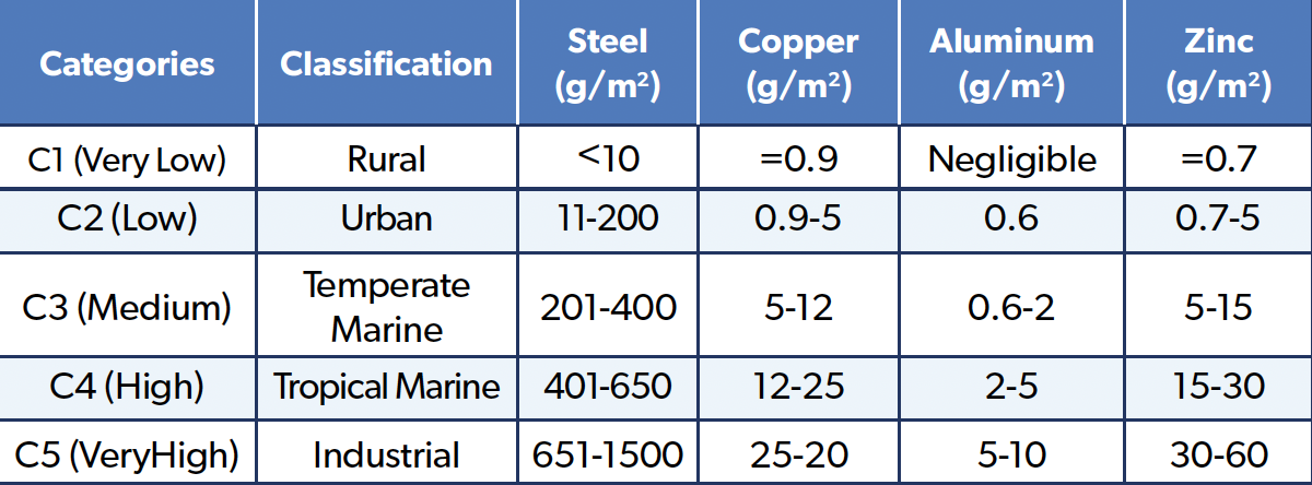
Canadian Arctic and sub-Arctic sites; Kucera et al. [9] in Scandinavia; and Mikhailov et al. [10] in eastern Siberia have shown corrosion rates of carbon steel close to the C1 category of the ISO 9223 classification (Table 1).

Table 1: One-Year Corrosion Rates and Corrosion Categories.

Even though the corrosion rates are lower than the C1 category, the substantial human growth and climate change in the Arctic and sub-Arctic region push that envelope. Because of this, there is a case to add a cold climate category to the classification. Factors that drive the atmospheric corrosion in cold climates are winds that can bring in salt-laden snow from the marine environment, and the use of de-icing salts can also contribute to high levels of chlorides [2]. The eutectic point, or the freezing point, of de-icing salts can be lowered to -50°C, melting the ice/snow layer on top of metal samples [7]. This phenomenon keeps metal samples moist for much longer periods, thus increasing the time of wetting (TOW).

In the presence of chlorides and moisture, extensive atmospheric corrosion damage can be observed on metal samples. Another contributing factor to high corrosion rates is low rainfall, which in turn cannot periodically wash off the deposited chlorides and SO2 on top of the samples [2]. In addition, ever-increasing ambient temperatures due to climate change in recent years affect the snow presence on top of the metal samples [11]. The temperature of the samples is not too high to evaporate the deposited snow/ice but high enough to cause melting and sustain moisture for longer periods of time. This leads to the formation of varying thicknesses of wet ice/snow layers on the metal surface. Long hours of sunlight in the summer also increase the surface temperature of metal samples beyond the ambient temperatures, causing dew formation and condensation, which in turn results in higher TOW.

Multi-Angle Test Rack Design

The design and methodology of atmospheric corrosion test racks have been guided by several pivotal standards over the years.

Prominently, the ASTM standard G50: “Standard Practice for Conducting Atmospheric Corrosion Tests on Metals,” and more particularly subsection five concerning exposure racks and frames, has served as an instrumental reference point for this research herein [12]. Similarly, ISO 8565, “Metals and alloys—Atmospheric corrosion testing—General requirements for field tests,” was another crucial standard consulted during the design process [13]. Over time, atmospheric corrosion test racks have seen iterative developments to address specific research requirements. Notable research endeavors that have trod a similar path include studies conducted in diverse geographies.These studies offer a comparative perspective and serve as benchmarks for the current investigation. A seminal study from 1995 introduced an atmospheric test rack design that facilitated specimen exposure across various orientations and angles [14].

Subsequently, a research team from the University of Hawaii devised the “Compact Octagonal-Prism Portable Exposure Rack” (COP-PER) to specifically assess the impact of wind direction and specimen orientation on corrosion rates [15]. Additionally, collaborative efforts from Spain and Portugal resulted in the development of a tree-shaped rack, designed to concurrently evaluate specimen orientation and exposure angle in atmospheric corrosion studies [16].

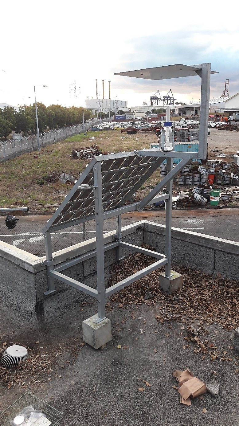
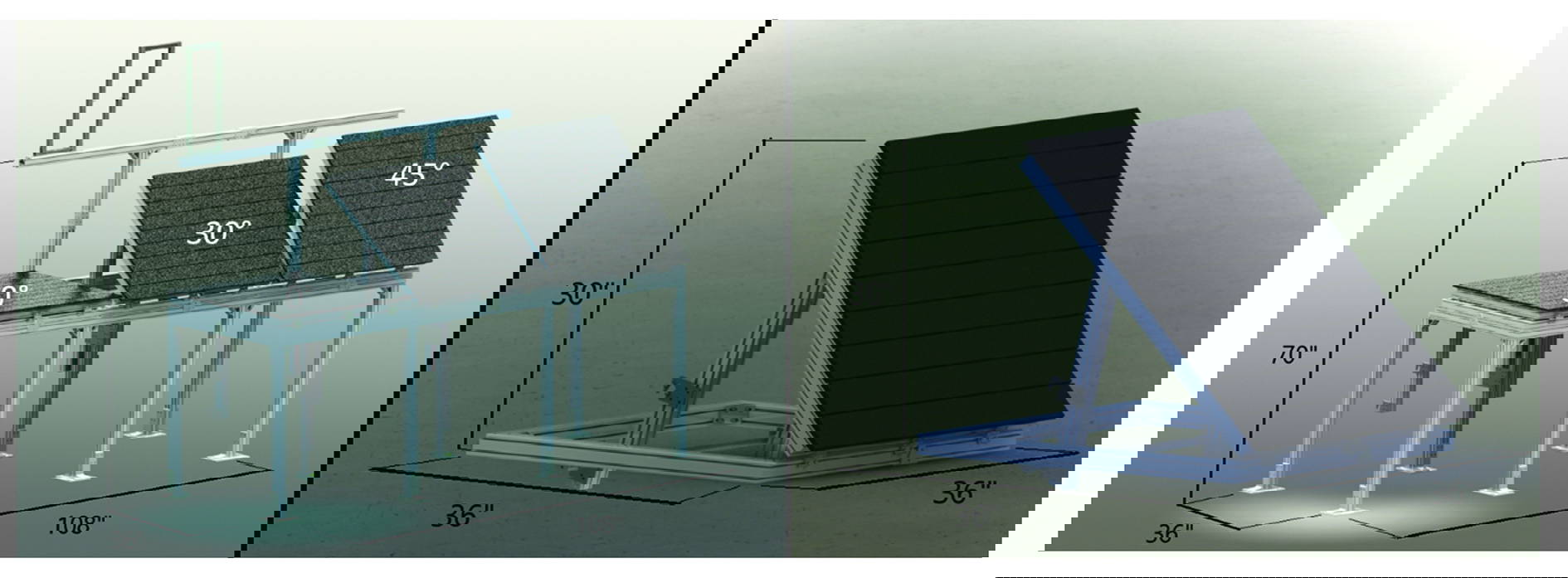
Traditional test racks used for atmospheric corrosion monitoring are often inadequate for Arctic deployment. They cannot withstand snow loads, high winds, or severe temperature swings. To address this, a modular and adjustable atmospheric corrosion test rack was designed, later patented in the United States as US 11,499,909 B2. The rack design includes adjustable exposure angles (0°, 30°, 45°), a modular aluminum frame, integrated sensors, and corrosion-resistant construction (Figure 1).

Figure 1: Adjustable Multi-Angle Corrosion Test Rack.

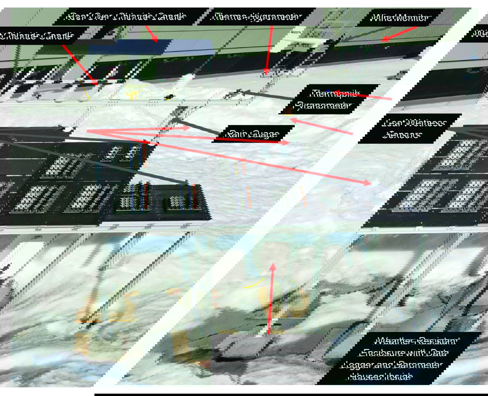
Atmospheric corrosion standards recommend an exposure angle of 30 degrees from the horizontal, facing south, and the lowest specimens be at least 30 inches above the ground. Time of wetness is one of the main parameters for atmospheric corrosion testing and can vary drastically depending on the angle of the exposed surface. This modular and adjustable corrosion test rack allows us to change the direction of exposure (north, south, east, or west) and the angle of exposure (0, 30, or 45 degrees to horizontal). These changes can be made easily and will save time when future adjustments are required for different exposure angles and directions. Lastly, this design can support a full weather monitoring system (Figure 2). These parameters include, but are not limited to, relative humidity (RH), ambient air temperature, TOW, rainfall, wind velocity, UV radiation, barometric pressure, and aerosol chloride and sulfate deposition.

Figure 2: Multi-Angle Corrosion Rack with Auxiliary Weather Station.

Establishing Test Sites

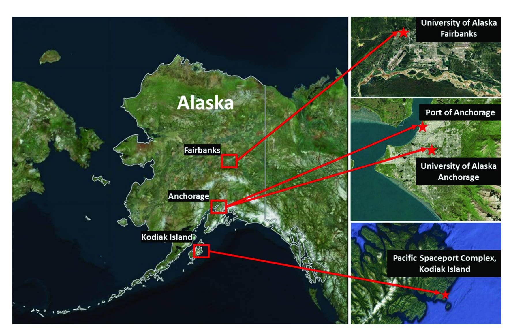
Four strategic locations were selected as preliminary testing sites, with site selection and characterization heavily influenced by ASTM G92 “Standard Practice for Characterisation of Atmospheric Test Sites” [17]. Their positions can be referenced in Figure 3, which provides a map of Alaska.

Figure 3: Map of Alaska Showing Four Corrosion Monitoring Sites.

Kodiak, AK – Pacific Spaceport Complex (PSCA) – Aggressive Marine Environment

Kodiak, AK, represents the aggressive marine environments commonly found along the southern and southeastern coastlines of Alaska. Coastal cities, such as Kodiak, receive on average a steady coastal breeze averaging 9 knots (4.6 m/s), average yearly precipitation of 65 inches (1651 mm), and average ambient temperatures of 41°F (5°C). This creates an aggressively corrosive

environment with relatively steady electrolyte exposure from rainfall and high relative humidity levels, as well as steady prevailing winds that provide high deposition rates of aerosol-borne Cl.

During the summer months, Kodiak experiences a maximum daily sunlight period of approximately 16 hours at the summer solstice and a minimum of 6.5 hours at the winter solstice. Both the summer and winter solstice are indicative of the maximum and minimum number of sunlight hours, respectively. This provides for periods of consistent solar irradiance exposure, which are maximized during the summers in Alaska. The exact exposure site is located in close proximity to the Pacific Spaceport Complex on Kodiak Island. Using pre-existing structures places the exposure rack ~5-6 feet elevated from the ground level and ~600 feet from the open ocean water.

Anchorage, AK – University of Alaska Anchorage (UAA) – Mild Marine Environment

Of the two exposure sites operated in Anchorage, AK, one resides at the University of Alaska Anchorage (UAA) and represents a very mild marine environment. Positioned 25 miles farther north than Kodiak, this site presents colder average temperatures and lower average precipitation rates comparatively. The average ambient temperature in Anchorage is 39°F (3.9°C) with an average precipitation of 16.9 in (430 mm). Both Anchorage sites typically exhibit lower average levels of relative humidity and receive lower Cl- deposition rates than those of Kodiak, but still experience these coastal effects, being only slightly offset from the shoreline.Anchorage sites receive longer periods of daily sunlight exposure, reaching upwards of 18.5 hours at the summer solstice and lowering to 5.5 hours at the winter solstice. This again provides generous solar irradiance exposure that is maximized during the summer months. At UAA, the particular exposure site is positioned on a building roof and is therefore elevated above the ground floor by ~30-45 feet. The site is also positioned much farther from the shoreline of the neighboring head of both the Knik and Turnagain Arm by ~4 miles. Where Kodiak is positioned far from any industrial or urban environment, UAA is positioned only a couple of miles from the downtown center. UAA is therefore more apt to be influenced by associated factors with urban areas, such as vehicle emissions and combustion byproducts, among others.

Anchorage, AK – Port of Alaska (POA) – Moderate Marine Environment/Mild Industrial Environment

The second of the two exposure sites, which operates in Anchorage, AK, resides at the Port of Alaska (POA, or “The Port”) and represents two environmental types with varying positions. Being situated similarly to the UAA site, all of the previous meteorological averages and data also apply to this site. The Port of Alaska handles the majority of fuel and freight cargo in Alaska, and it is an understatement that it is the lifeline of the Alaskan people. Its proximity to the ocean and constant truck movements make the Port of Alaska a strategic location to collect atmospheric corrosion data. In summary, upon inspection, the site presents a less corrosive environment than Kodiak does, with ample summer time solar irradiance exposure.

Fairbanks, AK – University of Alaska Fairbanks (UAF) – Inland Urban Environment

The last site is operated in Fairbanks, AK, at the University of Alaska Fairbanks (UAF), which best represents an inland urban environment. The summers are warmer than both Anchorage and Kodiak, with an average temperature of 60°F (15.6°C). However, the winters are much colder, with average winter temperatures of -4.3°F (-20°C). Average annual precipitation levels are the lowest of the four sites at 12.4 in (~315 mm). Fairbanks, being situated in a more northern location than Anchorage, receives exceptionally long periods of sunlight during the summer months, exceeding 21 hours at the summer solstice.

During winters, the inverse occurs with a mere 4 hours of sunlight at the winter solstice. This provides an incredibly large amount of solar irradiance exposure during the summer months relative to the other sites. Due to Alaska’s sheer size, Fairbanks lies approximately three hundred miles (~500 km) away from the nearest coastal area, which provides quite radical and unique weather challenges during the winter months. The particular site lies atop the Usibelli Engineering Building at approximately four stories, thus elevating the exposure rack ~60–72 feet above the ground floor.

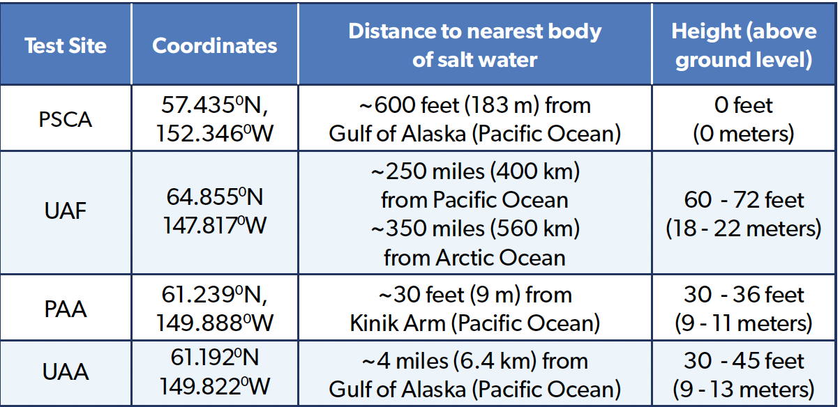
While the exposure to airborne Cl- and SO4²- is expected to be considerably lower than at 28 Kodiak due to the relative positioning from open bodies of salt water, respectively, the UAF exposure site does typically experience an elevated exposure to airborne SO4²-. Interior Alaska is abundant in individual residential heating solutions for the winter months. The most common combustion sources include heating oil and wood. Both produce either primary or secondary SO4²- within the atmosphere, with primary SO4²- generally making up the most significant percentages. Fairbanks’ geographical characteristics are also highly conducive to frequent temperature inversions during winter. Temperature inversions most often cause cold air masses to settle beneath larger warm air masses. In effect, this traps any and all airborne contaminants within the lower-lying cold air masses. Trapped contaminants then have a longer period and a chance to deposit on the sample surfaces. Additionally, UAF also sits across the street from the University Power Plant. Table 2 gives a detailed layout of each test location and geographical coordinates.

Table 2: Test Sites’ Coordinates, Distance From Sea, and Elevation.

Some Notable Results and Trends

Figure 4 delineates the ambient air temperature at the PSCA site, which, during the winter months, dips below the freezing mark on several instances and occasionally falls beneath -5°C. Despite these sporadic plunges, the overall trend captured by the solid red line indicates that the ambient air temperature stays above 0°C throughout the entire year-long exposure period, with the mean average, illustrated by the dotted red line, stabilising around 6°C. The PSCA’s proximity to the Pacific Ocean, a mere 600 feet away, confers a stabilising effect on its air temperature, moderating the extremes that might otherwise be observed. The climatic profile of Fairbanks, Alaska, is characterised by its starkly contrasting temperatures, with intense cold in the winter and, unexpectedly, notable warmth in the summer. As depicted in Figure 5, the ambient air temperature at the UAF site plummets to a frigid -35°C in December 2022 and soars to 28°C by late June 2022.

Figure 4: Ambient Air Temperature at PSCA – Raw vs Averaged Data. Figure 5: Ambient Air Temperature at Fairbanks – Raw vs Averaged Data.

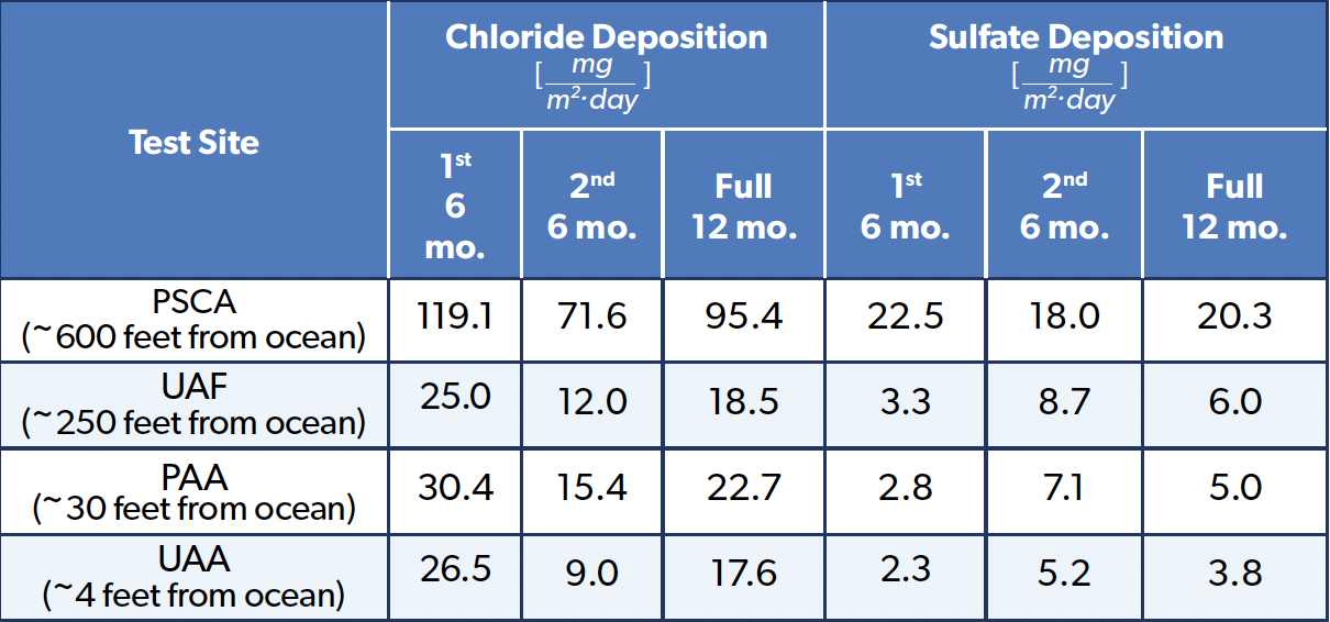
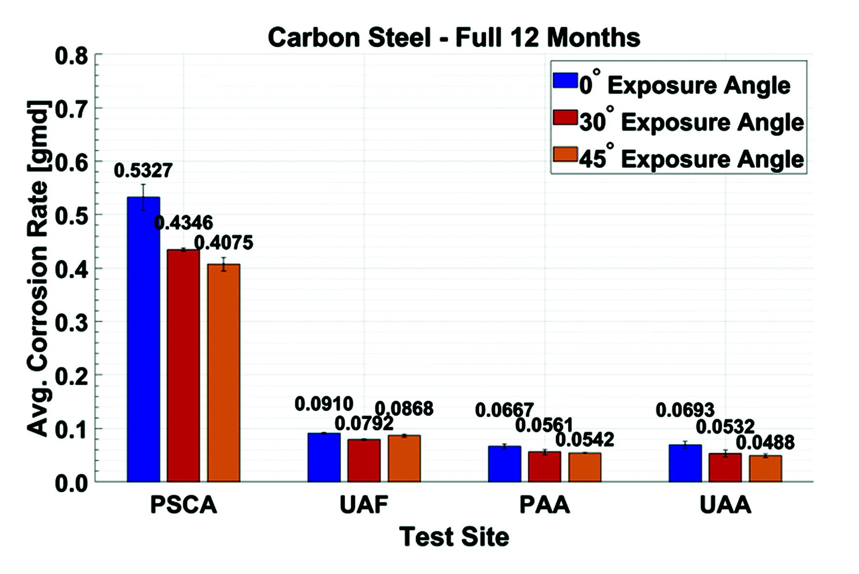
Table 3 shows the calculated chloride and sulfate deposition rates for each test site over each exposure. The PSCA site has four to seven times the amount of chlorides when compared to UAF and UAA, the PAA test sites. Figure 6 depicts the corrosion rates for 1008 carbon steel (UNS G10080) for a 12-month exposure period. The carbon steel samples at the PSCA site exhibited corrosion rates at least four times greater than the carbon steel samples exposed at UAF, PAA, and UAA.

This can be attributed to the weather data, where PSCA recorded at least four times the amount of chloride deposition, and the samples spent at least 18% more time wet through all sites and exposures. At the PSCA site, a distinct correlation was observed between the exposure angle and corrosion rate. Samples exposed at 0° showed the highest corrosion rates, followed by those at 30°, with the lowest rates seen at 45°. The TOW data indicates that the 0° angle samples remained wet for longer periods compared to 30° and 45°. Although the other sites – UAF, PAA, and UAA – exhibited less pronounced trends and experienced four times less corrosion than PSCA, the samples at 0° consistently showed higher corrosion rates than those at 30° and 45°.

Table 3: Chloride and Sulfate Deposition Rates.

 Figure 6: Average Corrosion Rates of 1008 Carbon Steel Over Full 12-Month Exposure Period.

Corrosion Rate Conversion

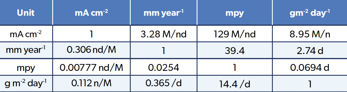
The following table is useful to put the above corrosion rates into context for the four test regions above.

Table 4: Corrosion Rate Conversion. 

Conclusion

New and innovative multi-angle corrosion test racks, each with auxiliary weather stations, were established at four test sites spanning across Alaska, USA. Each of Alaska’s four test sites presents a distinct corrosion profile: Kodiak (PSCA) exhibits high chloride-driven corrosion, Anchorage (PAA/UAA) faces freeze-thaw cycles with de-icing salts, and Fairbanks (UAF) experiences frost-dew cycling. Initial field campaigns revealed a clear correlation between exposure angle and corrosion rate. The combination of urbanisation and proximity to marine environments makes Arctic and sub-Arctic regions in North America, particularly Alaska, an important natural laboratory to study atmospheric corrosion in cold regions and the development of predictive models and corrosivity maps tailored for Arctic conditions. The fundamental knowledge of studying the basic atmospheric corrosion mechanisms in extreme cold conditions will result in better design practices for the built environment in the changing Arctic.

Acknowledgements

The author acknowledges the UAA’s College of Engineering and ConocoPhillips Arctic Science and Engineering Endowment, NASA EPSCoR CAN grant, and the many undergraduate students and collaborators who contributed to the design, installation, and operation of the corrosion monitoring sites across Alaska. Special thanks to graduate students Mr Tyler Cushman, Mr Jozef Huner, Mr Lawrence Giron Jr., Mr. Jacob Bodolosky, and machinist Mr Corbin Rowe. The author also gratefully acknowledges the organizations that provided access and site space for test rack installation, including the Pacific Spaceport Complex–Alaska (Kodiak), the Port of Alaska, the University of Alaska Anchorage, and the University of Alaska Fairbanks.

References

1. E A Wright, CRREL’s First 25 Years: 1961–1986, US Army Cold Regions Research and Engineering Laboratory, Hanover, NH, 1986.
2. Revie Winston (2000) Uhlig Corrosion Handbook, 2nd Edition.New York: John Wiley & Sons, Inc
3. ASTM Committee G1 “Corrosiveness of Various Atmospheric Test Sites as Measured by Specimens of Steel and Zinc,”in Metal Corrosion in the Atmosphere, ASTM STP 435, American Society for Testing and Materials, Philadelphia, PA, 1968, 360–391.
4. A Pearce and C G Smith, The Hutchinson World Weather Guide, Hutchinson, London, 1984.
5. J R Divine and L D Perrigo, “Atmospheric corrosion testing in the arcticand subarctic—a review,” Paper No. 389, in Proceedings of the Corrosion 86 Conference, NACE, Houston, TX, 1986.
6. P Sereda, “Weather Factors Affecting Corrosion of Metals,” in Corrosion in Natural Environments. ASTMSTP 558, American Society for Testing and Materials, Philadelphia, PA, 1974, pp. 7–22.
7. G W Brass, “Freezing depression by common salts: implications for corrosion in cold climates,” in Proceedings of the National Association of Corrosion Engineers, Canadian Region Western Conference, Anchorage, Alaska, 1996, pp. 447–453.
8. G A Biefer, Perform., 20(1), 16 (Jan. 1981).
9. V Kucera et , “Corrosion of Steel and Zinc in Scandinavia with Respect to the Classification of the Corrosivity of Atmospheres,” in S.W. Dean and S. Lee (Eds.), Degradation of Metals in the Atmosphere, ASTM STP 965, American Society for Testing and Materials, Philadelphia, PA, 1988, pp. 264–281.
10. A Mikhailov, M Syloeva, and E Vasilieva, Data Base on Atmospheric Corrosivity in Towns and Industrial Centres in the Territory of the Former USSR, Institute of Physics and Chemistry, Russian Academy of Science, Moscow,
11. A A Mikhailov, P V Strekalov, and Yu M Panchenko, “Atmospheric corrosion of metals in regions of cold and extremely cold climate (a review)”, Protection of Metals, 2008.
12. ASTM G50, “Standard Practice for Conducting Atmospheric Corrosion Tests on Metals,” ASTM International, doi: 10.1520/G0050-20.
13. ISO 8565, “Metals and Alloys. Atmospheric Corrosion Testing. General Requirements,” BSI Standards Limited, 2011.
14. Coburn, M Komp, and S. Lore, “Atmospheric Corrosion Rates of Weathering Steels at Test Sites in the Eastern United States — Effect of Environment and Test-Panel Orientation,” in Atmospheric Corrosion, 100 Barr Harbor Drive, PO Box C700, West Conshohocken, PA 19428-2959: ASTM International, 1995, pp. 101-101–13.
15. L H Hihara, J Kealoha, and N Das, “Studying the effect of wind direction and specimen orientation on the corrosion of 1018 steel using a compact octagonal prism portable exposure rack,” NACE, 2019.
16. J J Santana, et , “The influence of test-panel orientation and exposure angle on the corrosion rate of carbon steel. mathematical modelling,” Metals (Basel), vol. 10, no. 2, p. 196, Jan. 2020.
17. ASTM G92, “Standard Practice for Characterisation of Atmospheric Test Sites,” ASTM International, 2020.

Ivano Magnifico, Certified Senior Technician in Cathodic Protection.

Meet the Author
Ivano Magnifico holds a master’s degree in Electronic Engineering and serves as the Gas and Oil Product Manager at Automa, an ICorr Corporate Member.

A certified Cathodic Protection Specialist, he combines technical competence with deep knowledge of market analysis and industry standards. With over 15 years of experience in remote cathodic protection monitoring and a patent for an intelligent reference electrode, Ivano has made significant contributions to the field. He is a member of the Board of Directors of CEOCOR (European Committee for the Study of Corrosion and Protection of Piping Systems) and serves as the Delegate of the AMPP Italy Ivano Magnifico Chapter. In addition, he is an active participant in ISO and AMPP standard working groups on cathodic protection.

Introduction

The risk of AC corrosion has always been linked to the parallelisms of underground pipelines with High Voltage AC lines, especially in those geographical areas where the morphology of the territory creates obligatory so-called “technological corridors” and therefore forces the coexistence of different services over long distances.

Recently, the greater diffusion of AC-powered railway networks has further increased the AC interfering sources, while the use of more performing coatings on underground pipelines has on the one hand increased their insulation from the surrounding soil, and on the other has increased the risk of overprotection compared to old, less performing, or more degraded coatings.

This paper, starting from a real case found in a gas distribution network, will present the normative criteria to be used to keep
the AC corrosion risk under control, and will highlight how the simultaneous presence of cathodic overprotection may result in an autocatalytic cycle leading to accelerated AC corrosion, in which monitoring becomes essential in order to be able to carry out on time the appropriate corrective actions.

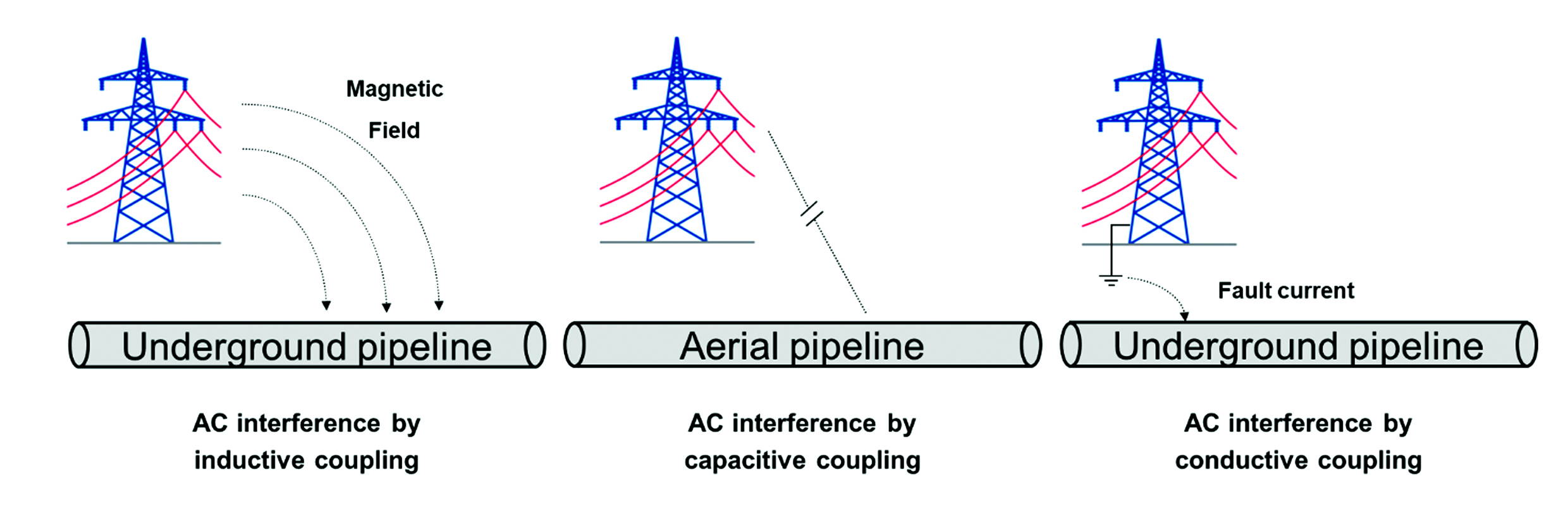
There are several mechanisms through which an AC source can interfere with a metal structure (Fig. 1): by inductive coupling,
as an effect of the magnetic field generated with respect to an underground structure; by capacitive coupling, in the case of an aerial structure; and by conductive coupling in the presence of a fault current in the ground, in the case of an underground pipeline.

In the case of underground pipelines, under normal operating conditions, the mechanism that can generate AC interference is inductive coupling: normally the interference effect is greater as larger the length of the sections where the pipeline and the AC source (high voltage AC lines, railways operated in AC) follow a parallel path.

AC Corrosion Protection Criteria

International industry standards specify which electrical parameters shall be monitored and their maximum allowed values. The standard ISO 18086:2019 “Corrosion of metals and alloys – Determination of AC corrosion – Protection criteria” indicates two steps for the verification of permissible AC interference levels (Fig.2):

Figure 1: AC Interference Mechanism.

Figure 2: AC Corrosion Risk Assessment According To ISO 18086.

The first step relates to a safety criterion for maximum permissible touch voltage (15V threshold) and does not have a direct rule in AC corrosion risk assessment. This value considers a hand-to-hand or hand-to-foot resistance for an adult male human body of 1500 Ω, yielding a current flow of 10 mA when 15 V is applied [2].

The criterion is based on current density measurements carried out through a coupon whose surface is defined by the standard to be 1 cm², connected to the structure. Both AC current density and DC current density must be measured, as the level of cathodic protection can affect the AC corrosion phenomenon.

NACE standard SP21424-2018 “Alternating Current Corrosion on Cathodically Protected Pipelines: Risk Assessment, Mitigation, and Monitoring” [3] expresses similar values, where depending on the measured DC current density (J.dc) value, different levels of AC current density (J.ac) are allowed:

• If J.dc > 1 A/m2 then J.ac < 30 A/m2; or
• If J.dc < 1 A/m2 then J.ac < 100 A/m2

This standard imposes a maximum AC current density limit even if the DC current density is less than 1 A/m², while the coupon surface of 1 cm² is indicated as generally used but not mandatory.
The Spread Resistance is the ohmic resistance through a coating defect towards remote earth and controls the DC (Idc) or AC (Iac) current passing through a defect at a given voltage (Udc or Uac):
Uac = R’s Iac or Uac = Rs J.ac (1)

where Rs is the normalized Spread Resistance expressed in Ω·m2.

On coating defects, where cathodic protection current reaches the steel surface, cathodic reactions occur involving oxygen reduction and hydrogen evolution. Both reactions generate hydroxide ions(OH-) leading to increased pH at the interface and alkalinity.

Since Spread Resistance depends [4] on both defect size (decreases as surface decreases) and pH value at the interface (decreases as pH increases), the DC current density reaching the defect affects it:

Lower current density leads to decreased pH value and increased Spread Resistance.

Higher current density leads to increased pH value and decreased Spread Resistance.

This is where overprotection can have an effect on AC corrosion:

Presence of a very electronegative IR-free potential (due to high DC current densities);

• Decrease in the Spread Resistance value;

• Possibility of significant AC current density even with low measured AC voltage.

Regarding the choice about which size of coupon to use, increasing the surface area of the coupon results in a lower average current density since the spread resistance increases linearly with increasing defect diameter and the current density decreases linearly with surface area.

Therefore, the current density is typically underestimated when the surface area of the coupon is chosen to be larger than the maximum defect size on the structure: for this reason, in the case of AC corrosion, the standards indicate the use of a 1 cm2 coupon.

AC Corrosion Mechanism in the Presence of Over-Protection [3]

For pipelines with applied cathodic protection, AC corrosion development requires simultaneous coexistence of induced AC, excessive cathodic protection, and small coating defects. Under these conditions:

1. Induced alternating current leads to alternating current discharge on coating defects.

2. AC current density is regulated by alternating voltage and spread resistance associated with the coating defect, through Ohm’s law.

3. Spread resistance depends on:
a. Coating defect size.
b. Soil resistivity near the defect.
c. Soil chemistry.
d. Cathodic protection current density in the coating defect.

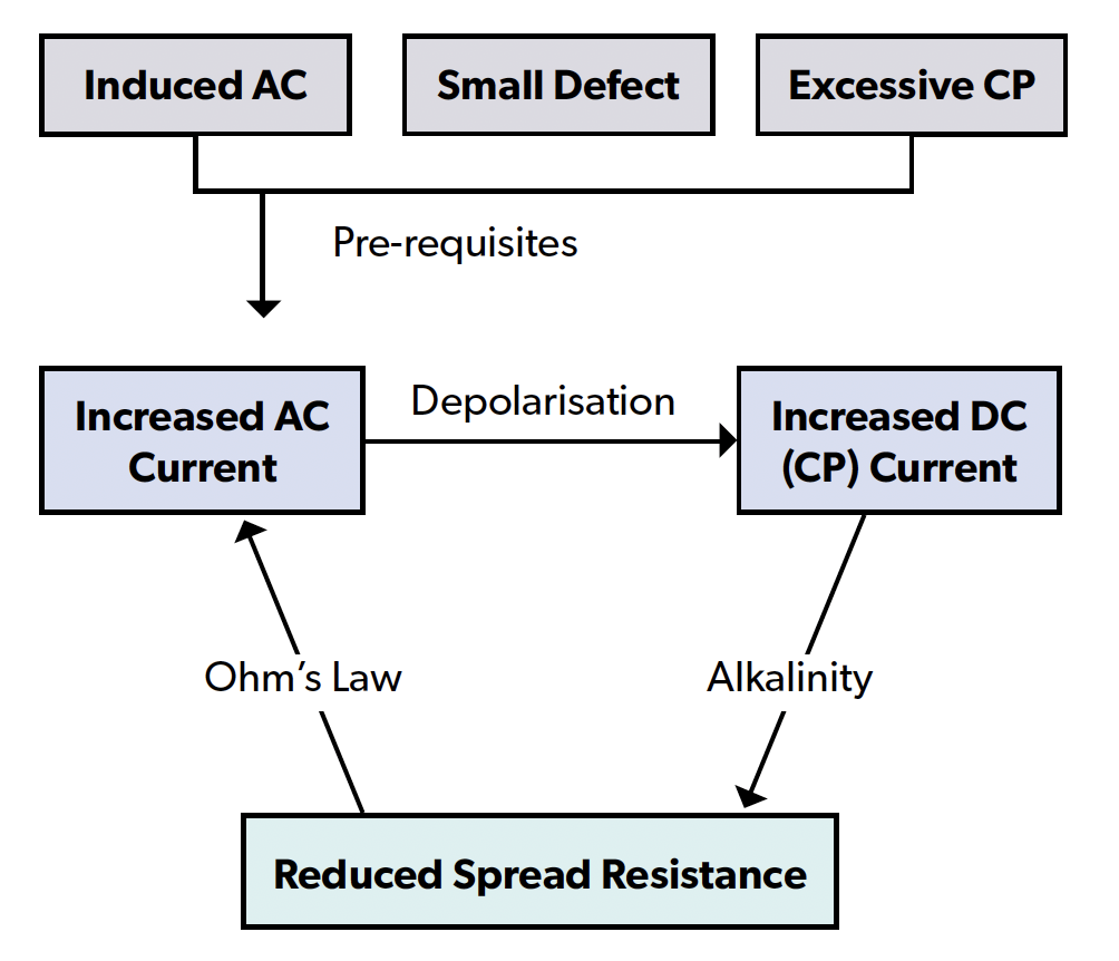
Figure 3 – Autocatalytic Nature of AC Corrosion on Cathodically Protected Pipelines Described by Sp21424.

As shown in Fig.3, the AC current density can lead to the depolarisation of the defect: this requires a higher DC current density to maintain a certain cathodic protection potential. Increasing the level of cathodic protection to mitigate AC corrosion, in this case, has the opposite effect: the increase in DC current density further decreases the Spread Resistance at the coating defect due to the production of OH- ions (alkalinisation). Through high levels of cathodic protection, the Spread Resistance decreases, thus increasing the density of alternating current, restarting the cycle: this scenario results in an autocatalytic cycle leading to AC corrosion.

It therefore becomes clear that, in order to leave this cycle, it is necessary to control both the AC current density and the DC current density.

Analysis of A Real Field Case

The case that will be shown has been detected on a measurement point of the distribution network of a large European city, with the following features:

• An extensive cathodic protection system forming a ring around the city center with radiating offshoots.

• Multiple crossings with DC powered railways and surface metro.

• Multiple parallels with the HVAC network.

• Cathodic Protection guaranteed by two T/Rs.

The analysed measuring point (MP):

• Located in a CP system area with several km of parallelism with HVAC line.
• Local soil resistivity between 25 and 50 Ω·m.
• Equipped with permanent CSE reference electrode with integrated 10 cm² coupon (measured current density is underestimated compared to 1 cm² coupon).
• Equipped with a G4C-PRO remote monitoring device capable of performing instant-off measurements on coupon and current density measures.

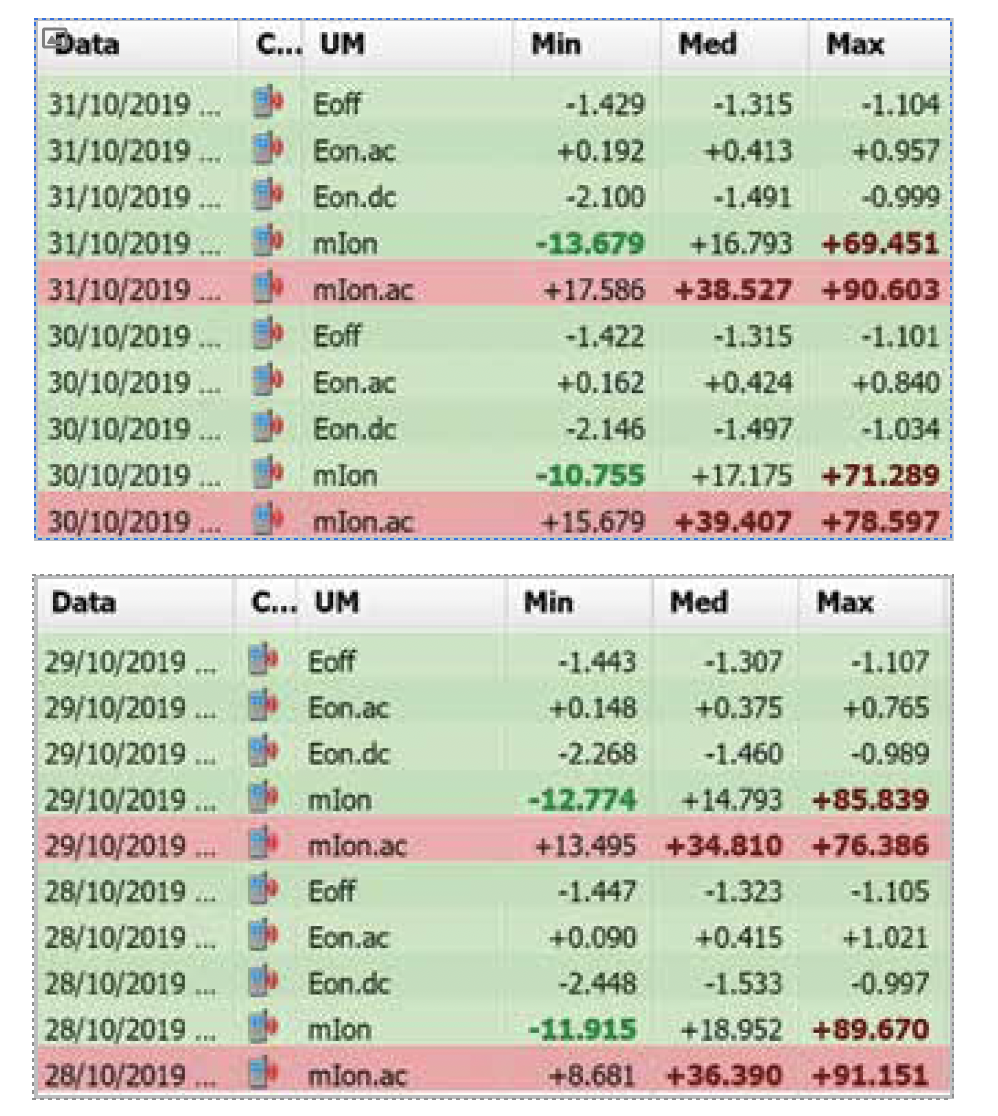
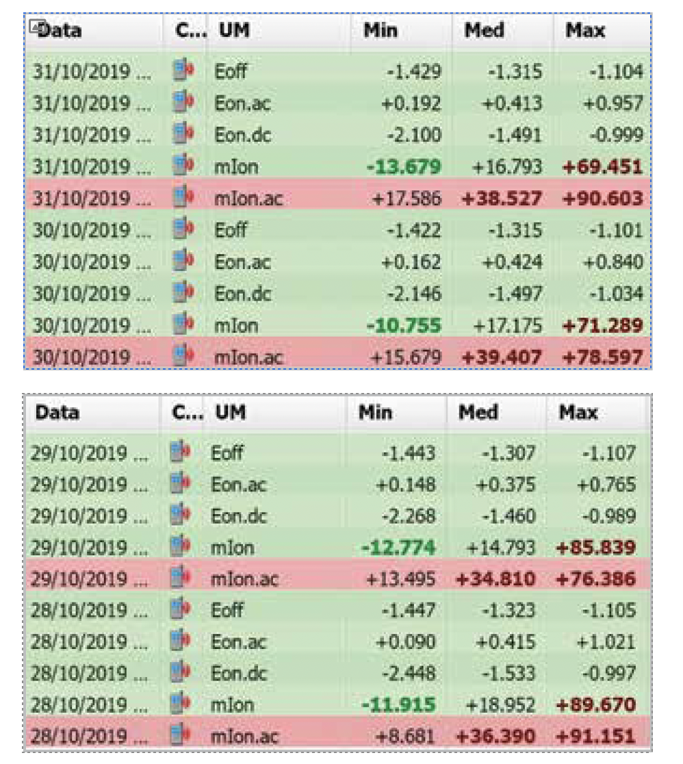
The measurements shown in Table 1 correspond to daily reports calculated on measurements performed continuously at a frequency of 1 Hz (1 measure per second) for each measuring channel. The minimum, average and maximum daily values are shown over a period of 4 days:

• Eon.dc: ON potential (DC) expressed in V CSE;
• Eon.ac: ON potential (AC) expressed in V;
• E off: instant-off on coupon, equivalent to IR-Free potential
(measured, every second, after a 1 ms wait from switch opening and over a 20 ms interval) expressed in V CSE;
• mIon: DC polarisation current of the coupon expressed in mA; as the coupon size is 10 cm2 the shown value corresponds to the current density in A/m2;
• mIon.ac: AC polarisation current of the coupon expressed in mA; as the coupon size is 10 cm2 the shown value corresponds to the current density in A/m2 (note: the current density value measured on a 1 cm2 coupon would be significantly greater than that measured on the 10 cm2 coupon).

In the absence of coupons, the only available measures would be Eon.dc and Eon.ac, and, on these values, the only possible evaluation would be that relating to the first step of ISO 18086, which would be absolutely respected considering that the highest AC average value along the four days shown (0,424 V) is well below the indicated threshold of 15V. Generally, such a low AC voltage value would never suspect a real risk of AC corrosion, but as can be detected from the DC and AC current densities, we are faced with unacceptable interference levels:

• mIon: between 15 A/m2 and 17 A/m2:

o greater than the threshold of 1 A/m2 for which (according to ISO 18086) the AC current density value would be indifferent.

• mIon.ac: between 35 A/m2 and 39 A/m2:

o greater than the threshold of 30 A/m2 indicated by ISO 18086 and NACE SP21424.

The explanation for this situation is given precisely by the significant level of cathodic overprotection present, represented by IR-Free potential values more negative than -1.3 V CSE and very high DC current density values, being the MP in a site suffering cathodic DC interference generated by metro and railway systems.

This results in a reduction of the Spread Resistance value, up to the point of generating an AC current density higher than the allowed limits even in the presence of a very low AC voltage.

The main evidence of the dependence of this condition on over-protection has been clearly shown when, due to a malfunction, one of the two T/Rs protecting the Cathodic Protection system did shut down, changing the values measured on the Measurement Point as in Table 2:

Hani Almufti, Technical Lead, Cogbill Construction (RedLineIPS), USA.

Meet the Author

Hani Almufti is Engineer and Manager of Strategic Development at Cogbill Construction (RedLineIPS), where he leads product strategy, materials selection, and technical guidance for metallic and non-metallic pipe support systems. He holds a B.S. in Industrial Engineering and is a Master’s candidate in the same field. With 15+ years in pipe supports—including a decade focused on offshore energy corrosion—he specialises in corrosion under pipe supports (CUPS) and the performance of FRP/composite and metallic supports. His expertise spans corrosion mitigation, reliability engineering, and process improvement, with a sustained focus on reducing risk, noise/vibration, and lifecycle cost across onshore and offshore assets.

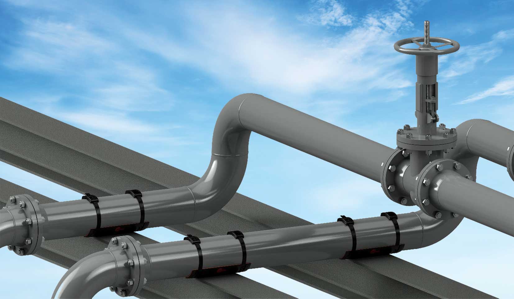
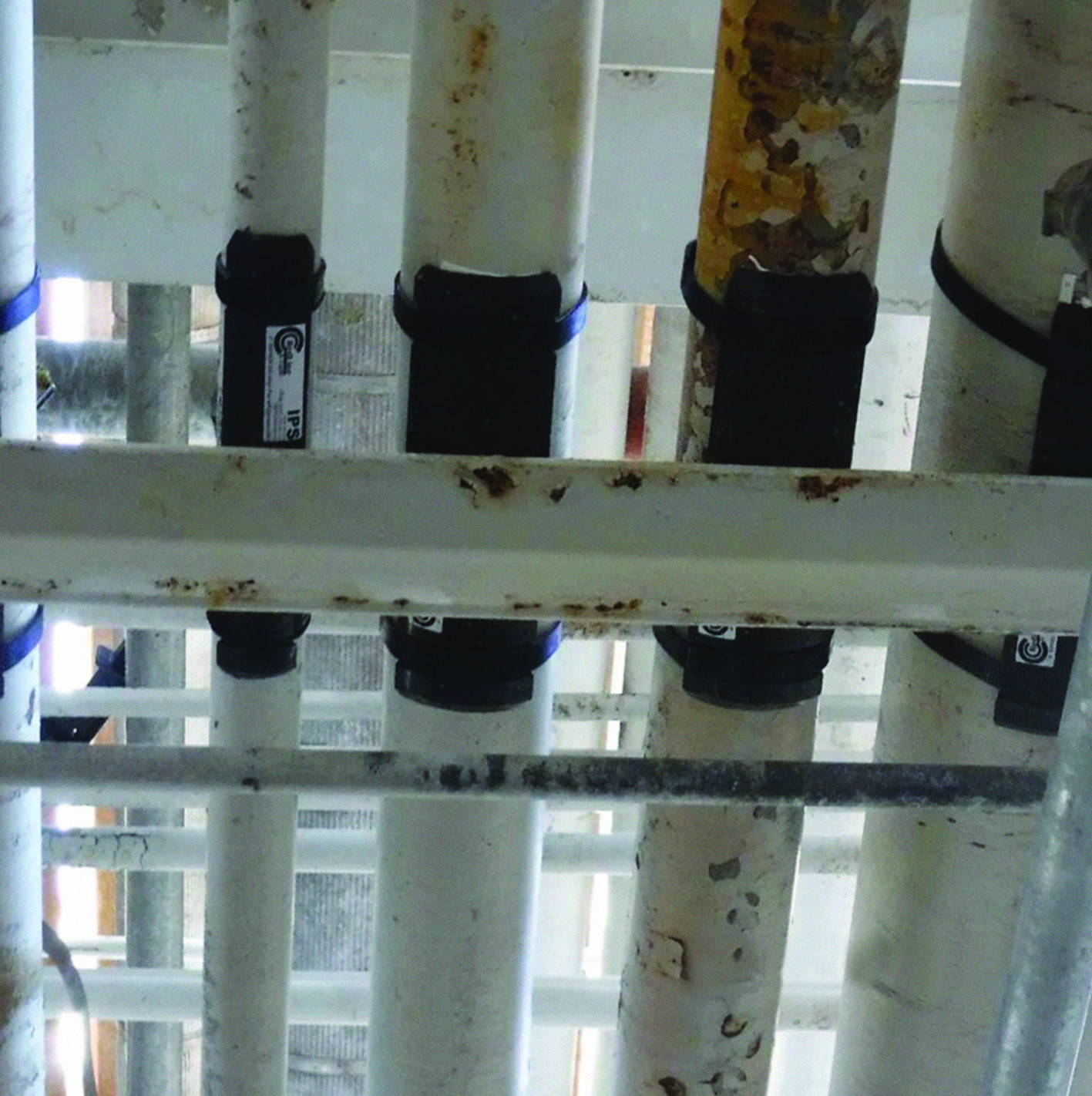
Photo 1: Installed System On Pipe Gantry.

1. Introduction

Pipe-support interfaces are convergence points for several degradation modes in industrial and offshore piping: corrosion under pipe supports (CUPS), vibration, structure-borne noise, and fatigue. On offshore platforms and FPSOs, major operators have reported that these risks are heightened by salt-laden atmospheres, hull motion, and restricted access, while the pipe–pad contact remains difficult to inspect [1].

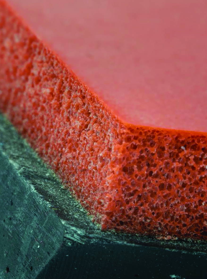
Conventional mitigations—welded metallic pads, thermoplastic half-rounds, and epoxy-bonded plates—can re-establish galvanic paths, trap electrolyte, or require hot work and cure time. Maintaining seal integrity, alignment, and controlled slip becomes increasingly challenging as coatings wear and thermal cycles accumulate [1]. The RedLineIPS SmartPad System is a fully non-metallic support interface comprising a load-spreading FRP saddle, a bonded closed-cell elastomeric gasket (Hydroseal), and FRP bands/buckles.

Together, they electrically isolate the pipe from the steel support, seal the pipe–pad contact to discourage moisture films, provide viscoelastic damping at the interface, and relocate thermal slip to a controlled, low-friction plane on the saddle/support side. This paper outlines the design rationale, installation approach, and third-party proofs, and summarises field experience from a Gulf Coast of Mexico chemical plant retrofit programme.

2. The SmartPad System

2.1 Composite FRP SmartPad (Saddle Wear Pad)
2.1.1 Construction and geometry
Structural fibre-reinforced polymer (FRP) saddle fabricated from continuous-strand mat (CSM) in a vinyl-ester matrix, moulded to standard pipe curvatures of 1/2” to 72” NPS. The crown radius and contact width are sized to spread load over a broad arc, keep local bearing pressure low, and maintain stable seating under thermal and dynamic loads.

2.1.2 Functions at the pipe–pad interface
• Load distribution: Spreads the pipe’s weight over a wider area so no small spot takes all the pressure—reducing dents and coating damage.

• Electrical isolation: Non-conductive composite interrupts metal-to-metal continuity (limits galvanic coupling to support steel).

• Coating protection: Smooth, inert bearing surface reduces abrasion during thermal slip and vibration.

• Offshore durability: Vinyl-ester chemistry with UV inhibitors tolerates chloride-rich, marine atmospheres.

Photo 2: SmartPad Exoskeleton with Grooves for Bands.

2.1.3 Typical Material Properties

• Resin system: Vinyl ester; reinforcement: CSM; glass content: ~35–40 wt%.

• Compressive strength (ASTM D695): ~25,000 psi
(172 MPa) [2].

• Flexural strength (ASTM D790): >30,000 psi (207 MPa).

• Continuous service temperature: -60°F to 400°F (-51°C to 204°C).

• UV resistance: High (integral inhibitors).

• Fire behaviour: Fire-retardant formulation (rating available on request).

2.1.4 Manufacture and Integration

Hand lay-up with controlled cure to achieve low void content and uniform fibre wet-out. Finished edge radii and surface roughness are controlled to minimize coating gouge. Saddle curvature and contact-width tolerances support repeatable fit and clamp preload. The FRP saddle provides the load-bearing, isolating substrate for the bonded closed-cell gasket and FRP banding within a fully non-metallic load path.

2.2 Hydroseal Closed-Cell Gasket

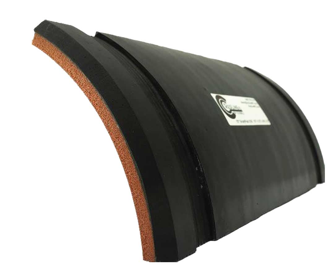
Photo 3: FRP Saddle and Closed Cell Gasket.

2.2.1 Construction and Placement

Factory-bonded to the SmartPad’s pipe side, the closed-cell elastomer compresses under band preload to form a continuous, conformal contact that accommodates normal surface roughness and remains uniform through thermal and vibration cycles at the pipe–pad interface.

2.2.2 Functions at the Pipe–Pad Interface

• Moisture Exclusion / CUPS Control: Very low water uptake; compressed contact suppresses crevice geometry and ion/oxygen transport, limiting crevice/under-deposit and MIC precursors.

• Vibration and Noise Attenuation: Viscoelastic damping lowers transmitted shear and micro-slip; the compliant, non-metallic layer acts as an acoustic impedance break to reduce structure-borne noise and alternating stress.

• Assists Galvanic Isolation: In combination with the FRP saddle, maintains a fully dielectric contact path.

2.2.3 Typical Material Properties

• Type: Closed-Cell Elastomer (e.g., silicone / EPDM)

• Density: 14–18 lb/ft³ (≈225–290 kg/m³)

• Compression-deflection @25% (ASTM D1056): ≈7.5 psi (≈52 kPa) [3]

• Hardness (ASTM D2240, Shore 00): 40–60

• Water absorption (ASTM D471): <0.1% by volume

• Operating temperature: –60°F to 570°F (-51°C to 300°C) • Compression-set resistance: Excellent

2.2.4 Durability and Integration

Under FRP-band preload, the gasket maintains stable compression, preserving seal and damping through thermal/vibration cycling and tolerating minor surface irregularities from prior repairs. Within the fully non-metallic load path, the gasket supplies sealing, compliance, and energy dissipation that complement the saddle’s stiffness and protect the coating at the pipe–pad interface.

2.3 SmartBands

2.3.1 Construction and Locking

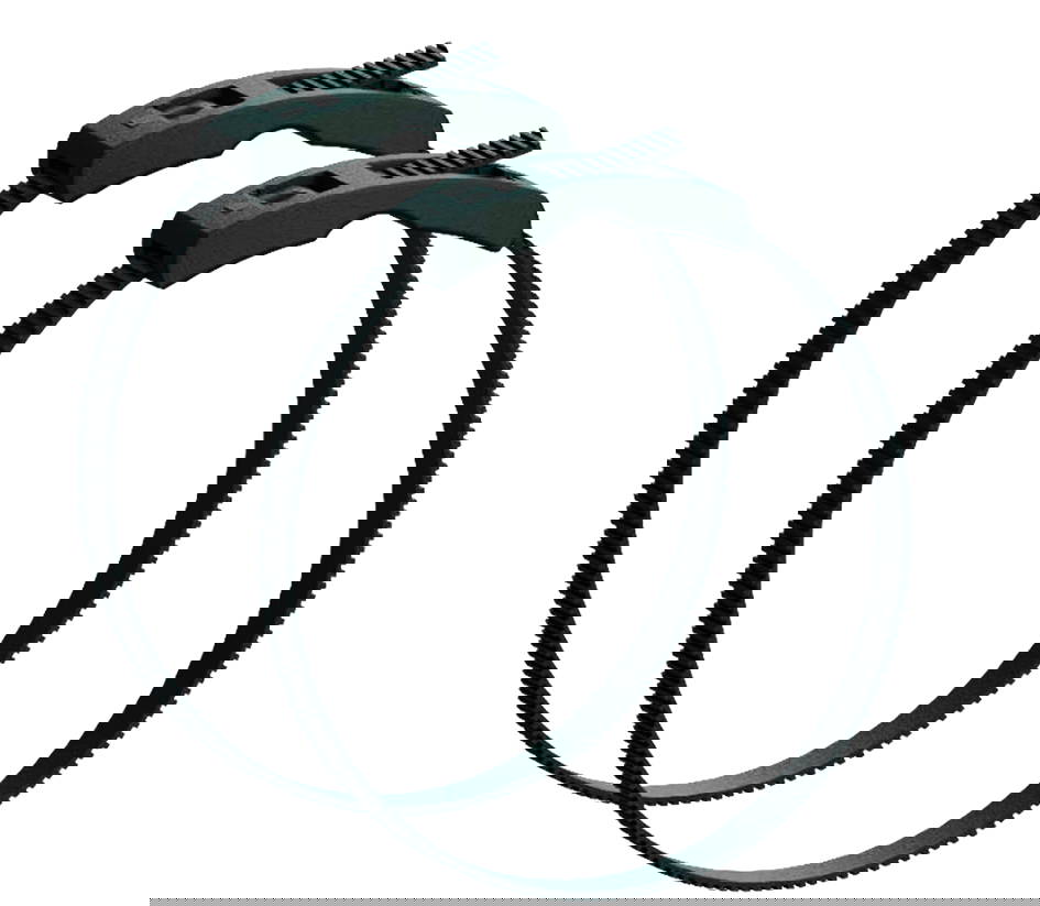
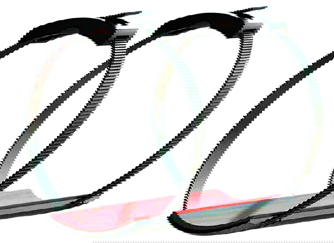
Continuous long-strand FRP straps in a UV-resistant resin, paired with a matching-pitch FRP square-tooth buckle for incremental, non-backdrivable engagement. Radiused edges and smooth faces limit stress risers and coating damage.

Photo 4: Non-Metallic Straps and Buckles.

2.3.2 Functions at the Pipe–Pad/Support Interface

• Dielectric clamping: All-composite load path preserves electrical isolation (avoids galvanic reintroduction).

• Preload delivery/retention: Long-strand reinforcement improves load transfer and creep/fatigue resistance, maintaining clamp force through thermal and vibration cycling.

• Surface compatibility / constructability: Non-marring inner face; smooth outer face for clean tensioning. Installs with a calibrated handheld tool—no hot work or adhesives.

2.3.3 Typical material properties

• Material: Continuous-strand FRP; UV-resistant resin.

• Tensile capacity (per band): ~1,200 lbf (≈5.3 kN).

• Thermal range: –40 °F to 250 °F (–40 °C to 121 °C).

• Electrical behaviour: Dielectric, non-metallic.

• Environmental durability: Corrosion-immune; outdoor/UV rated for coastal/offshore service.

2.3.4 Installation and Preload Control
Bands routed in moulded circumferential grooves in the saddle engage the FRP buckle and are tensioned to specification with a calibrated tool. Groove geometry sets bend radius, keeps the strap flush/recessed, and prevents lateral migration; the low-profile routing avoids snagging and maintains uniform bearing. Preload is confirmed by tool indication (or witness marks). For underside inspection, bands are single-use—they are cut and replaced with new bands; replacements are low-cost, and reinstallation typically takes minutes per support. Grooved routing also localises relative motion to the engineered slip plane at the saddle–support interface [4].

2.3.5 Durability and Integration
The continuous-strand architecture resists creep and tooth-root fatigue under cyclic loads. UV-stabilised resin supports long outdoor exposure; the all-composite assembly is unaffected by chloride corrosion. SmartBands provide the clamping force that maintains the Hydroseal seal and the saddle’s load-sharing contact within a fully non-metallic load path.

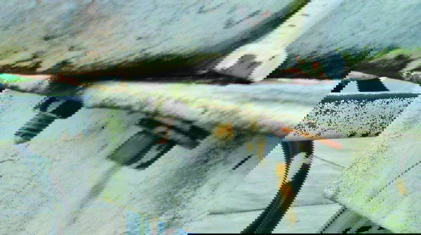
Photo 5: Example of Corrosion Under Pipe Support.

3. Corrosion Mechanisms at Support Interfaces

3.1 Crevice / Differential Aeration

Mechanism:  A narrow, shielded gap at the pipe–pad interface traps a thin electrolyte. Oxygen is depleted inside the gap while adjacent surfaces remain aerated, creating an anode/cathode differential. Wet–dry cycling concentrates chlorides and lowers pH, undermining coatings and accelerating localised metal loss [1].

SmartPad Mitigation: A factory-bonded, closed-cell Hydroseal gasket forms a continuous conformal contact under preload, denying voids where films persist. The FRP saddle spreads load to keep contact pressure uniform through thermal cycles, disrupting the differential-aeration cell associated with CUPS.

3.2 Galvanic at the Support

• Mechanism: Electrically coupled dissimilar (or conditionally different) metals sharing an electrolyte drive anodic dissolution; small-anode/large-cathode area ratios intensify attack at supports [1].

• SmartPad Mitigation: A fully dielectric load path—FRP saddle, Hydroseal gasket, and FRP SmartBands™/buckles—breaks metal-to-metal continuity. The sealed interface also limits shared electrolyte, cutting off both prerequisites for galvanic corrosion.

3.3 Microbiologically Influenced Corrosion (MIC)

• Mechanism: In intermittently wet crevices, biofilms (e.g., SRB) create chemically distinct microenvironments (sulfides, acidity, differential aeration) that localise attack

[1]. • SmartPad Mitigation: The low-uptake, closed-cell contact shortens wet-film residence time and reduces attachment sites. Smooth, non-porous, electrically isolating surfaces further discourage biofilm establishment and persistence at the pipe–pad interface.

3.4 Fretting-Assisted Corrosion

• Mechanism: Sub-millimeter relative motion from vibration/thermal cycling abrades coatings and oxides; freshly exposed steel corrodes between slips, forming a wear–corrosion feedback loop focused at the supports [1].

• SmartPad Mitigation: Viscoelastic damping in Hydroseal stabilises the pipe–pad contact and lowers micro-slip. Required thermal movement is relocated to the low-friction saddle–support interface, while the FRP saddle’s load distribution reduces shear at the pipe wall.

3.5 Under-Deposit/Capillary Thin-Film

• Mechanism: Deposits or capillary-held films trap chloride-rich, oxygen-poor moisture that behaves like a crevice beneath the footprint [1].

• SmartPad Mitigation: The bonded, continuous interface leaves no seam for solids to wedge; closed-cell elastomer resists wicking. Moisture remains on exposed, cleanable surfaces rather than beneath the pipe.

4. Vibration

4.1 Sources and frequency content
Piping vibration originates from rotating/reciprocating equipment (pumps, compressors, blowers), pulsation in positive-displacement services, turbulence at fittings/reducers, two-phase/cavitation, hydraulic transients, alignment/soft-foot issues, and support stiffness mismatches. Field spectra commonly fall in the 10–100 Hz band with ~0.25–2.5 mm (0.01–0.10 in) peak-to-peak motion; response amplifies near span/support natural frequencies (cf. ISO 20816-1) [5].

4.2 Why the pipe–pad interface matters
Rigid, metal-to-metal load paths transmit dynamic energy as micro-slip and contact shear at the pipe–pad interface. This accelerates coating wear (promoting CUPS), excites support steel (structure- borne noise), loosens hardware, and increases alternating stress Δσ—shortening fatigue life per S–N behaviour.

4.3 SmartPad mitigation mechanisms
• Interface damping (Hydroseal). The closed-cell elastomer provides viscoelastic damping in the 10–100 Hz range, reducing transmitted shear/micro-slip and smoothing contact pressures [6].

• Relocated slip (FRP saddle). The moulded saddle furnishes a controlled, low-friction slip plane at the saddle–support interface so thermal movement does not abrade the coating at the pipe–pad interface; broad bearing further lowers work per cycle.

• Stable dielectric clamping (SmartBands™ in recessed grooves). Calibrated, all-composite preload maintains uniform contact without re-introducing metallic short circuits, low-profile routing resists lateral migration and secondary rattles.

5. Sound (Structure-Borne Noise)

5.1 Mechanism
Dynamic forces excite the pipe wall; a rigid, metal-to-metal path at the pipe–pad interface transmits that energy into support steel and deck members, which then radiate airborne noise. Frictional micro-slip at a hard contact can also generate “stick–slip” (squeal) components. Acoustic transmissibility rises when the interface impedance closely matches the supporting structure.

5.2 Sources and Frequency Content
The same drivers as vibration—rotating/reciprocating equipment, pulsation in positive-displacement (PD) services, turbulence, two-phase/cavitation, hydraulic transients, alignment/soft-foot, and support stiffness issues—dominate. On process/offshore lines, most structure-borne content is ~20–200 Hz, overlapping habitability and communication bands

[5]. 5.3 SmartPad Noise-Control Mechanisms

• Impedance break + damping (Hydroseal): The closed-cell elastomer introduces a compliant, non-metallic layer at the pipe–pad interface, lowering mechanical impedance and adding viscoelastic loss. Result: reduced transmissibility and less friction-generated noise from micro-slip.

• Controlled slip on the support side (FRP saddle): The moulded FRP surface provides a low-friction slip plane at the saddle–support interface, keeping relative motion off the coating and suppressing stick–slip at the pipe–pad contact. Broad bearing further lowers contact forces that drive radiation.

• Dielectric, Low-Profile Clamping (SmartBands in recessed grooves): All-composite bands maintain the decoupled path
(no metallic short-circuit) and sit flush to avoid secondary rattles; calibrated preload keeps contact uniform.

6. Structural Integrity (Fatigue & Stability)

6.1 Overview
The pipe–pad interface largely governs fatigue performance at supports. A hard, rigid contact concentrates routine loads and transmits vibration into repeatable stress cycles, leading to local denting, coating loss, misalignment, and ultimately crack initiation in the pipe wall or supporting steel [7].

6.2 Principal contributors at supports
• Thermal restraint. Limited slip forces the pipe to bear against the interface; daily temperature swings add alternating load.

• Small real contact area / edges. Narrow bearings or sharp transitions elevate local pressure and seed dents.

• Dynamic excitation. Equipment- and flow-induced vibration increases the stress range each cycle.

• Fit-up variability. Misalignment or uneven bearing amplifies local stress and accelerates coating abrasion.

6.3 Why this matters for fatigue

Fatigue life follows S–N behaviour and is controlled by the alternating stress amplitude (Δσ). Dents, coating scrapes, and other stress raisers reduce cycles to initiation; once the coating is breached, corrosion further degrades the section, compounding risk [7].

6.4 SmartPad mitigation mechanisms

• Load distribution — FRP saddle. Broad bearing lowers peak contact pressure and mitigates edge effects; the non-conductive substrate avoids metal-to-metal paths that undermine coatings.

• Compliance & damping — Hydroseal gasket. A firm, closed-cell elastomer equalises contact pressure, absorbs vibration, and cushions small impacts, reducing contact shear and Δσ per cycle [6].

• Controlled movement without abrasion — saddle–support slip plane. Thermal growth is taken on the moulded FRP surface (optional low-μ liner if needed), minimising stick–slip and fretting at the pipe–pad contact.

• Stable alignment & clamp — SmartBands in recessed grooves. Calibrated, all-composite preload keeps contact uniform and resists lateral migration; the dielectric, low-profile routing avoids galvanic short-circuits and loose hardware.
(For underside inspection, bands are single-use—cut and replaced; this is a low-cost operation).

Photo 6: Full System Assembly.

7. Third-Party Testing: SmartPad Suitability for Industrial Service

Independent third-party testing was performed on specimens, as follows:

7.1 Results – Proof Loads, No Failures Observed

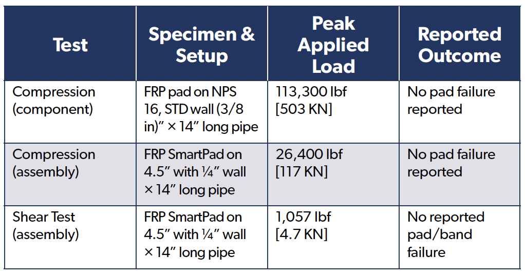
• Pad-only Compression: FRP saddle on NPS 16, STD wall pipe sustained 113,300 lbf axial compression without pad failure.

• Assembly Compression: Banded SmartPad-on-pipe (4.5 in OD × ¼ in wall) sustained 26,400 lbf axial compression without pad failure.

• Assembly Shear: Same assembly sustained 1,057 lbf lateral
(shear) without pad or band failure.

7.2 Interpretation
For the geometries/fixtures tested under monotonic loading, neither the composite saddle nor the banded assembly was the limiting element. The components tolerated high localised bearing and incidental lateral restraint typical of pipe-support reactions when installed and preloaded to specification.

7.3 Scope and Limits
These are static proof tests on short specimens. They do not establish design allowables or characterise fatigue, creep/relaxation, or environmental durability. Apply normal owner engineering practices (codes, load combinations, temperature, vibration/fatigue assessment) [8,9].

7.4 Implication for Use
Combined with the corrosion mechanisms described in section 3 (sealed dielectric interface, viscoelastic damping at the pipe–pad contact, and load spreading/controlled slip), the proofs support the SmartPad System’s mechanical suitability as a non-metallic pipe-support interface for industrial and offshore service, subject to project-specific engineering review.

8. Case Study — Coastal Texas Chemical Plant (Anonymised) Background

A large Gulf Coast complex retrofitted the RedLineIPS SmartPad System to mitigate CUPS, structure-borne noise, and nuisance vibration at pipe/support interfaces in a salt-laden, high-humidity environment.

8.1 Scope

• Units: Olefins recovery, utilities/cooling water, brine handling.

• Lines: Carbon-steel piping from 2”–24” NPS; cooling-water return, light condensate, brine.

• Quantity: ~5,000 supports installed during routine windows (no hot work).

• Configuration: FRP saddle + bonded Hydroseal closed-cell gasket + FRP SmartBands/buckles.

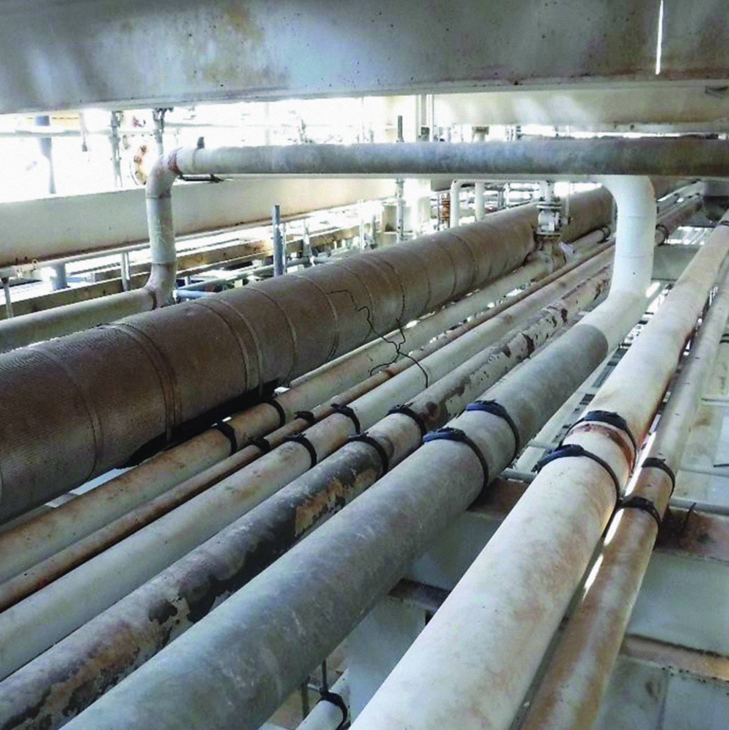
Photo 7: Installed System at Formosa Plant.

Photo 8: Installed System at Formosa Plant.

MEET THE AUTHORS

Dr Yifeng Zhang is a Postdoctoral Research Associate in the Non-Destructive Evaluation (NDE) Group at Imperial College London. His work focuses on ultrasonic Structural Health Monitoring (SHM) and inspection technologies that enhance structural integrity and operational efficiency across the energy and petrochemical sectors.

Dr Frederic Cegla is a Reader/Associate Professor in the non-destructive evaluation (NDE) Group at Imperial College London. His research focuses on developing and applying advanced technologies for non-destructive evaluation NDE, SHM, and process monitoring — linking cutting-edge sensing and wave physics with practical solutions for industry.

Introduction: The Challenge of Corrosion Surveillance

Corrosion remains one of the most persistent challenges in managing industrial assets such as power plants, processing facilities, pipelines, and ships. Unlike sudden failures, it develops gradually, often across vast areas and over decades of service.

The result is a degradation process that is both spatially and temporally diverse. Non-destructive evaluation (NDE) techniques such as ultrasonic testing and thickness gauging are widely used to provide critical information that underpins the safety, reliability, and availability of various assets. In practice, it is rarely feasible to perform complete (100%) inspection coverage of large downstream or marine facilities. Instead, inspection areas are typically prioritised using risk-based assessment (RBA) programmes, which focus resources on regions with the highest likelihood or consequence of corrosion Because of these practical constraints, current ultrasonic methods have evolved along two main directions.

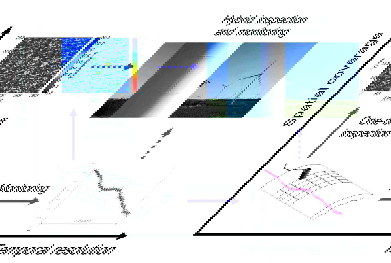
Figure 1: Ultrasonic Thickness Measurement Techniques, Trade-Offs Between Spatial Coverage and Temporal Resolution.

Scheduled one-off inspections — often combined with visual assessments and performed using scanning systems — can cover large areas but occur infrequently due to the need for plant shutdowns or limited access [1–2]. In contrast, permanently installed automated monitoring sensors offer improved measurement repeatability and high temporal resolution but are typically deployed only at a few selected locations [3–4] owing to cost and installation complexity.

Towards Hybrid Inspection and Monitoring

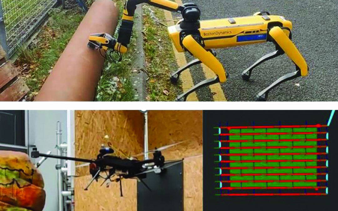
Recent advances in robotics and sensor technologies are creating powerful synergies that blur the line between traditional one-off inspection and continuous monitoring. It is envisaged that autonomous robotic platforms will in future manipulate ultrasonic probes across complex geometries, while monitoring sensors will be deployed in hard-to-reach areas that once required significant manual effort.

Prototypes of resident inspection robots — designed to remain on the asset and operate semi-independently — are moving from research labs towards field demonstrations [5-6].

Figure 2: Integration of EMAT With Robotic Platforms (Image Courtesy of The Offshore Robotics for The Certification of Assets (ORCA) Hub, From Research That Led To The Formation of Sonobotics Ltd).

These developments point towards a hybrid surveillance model that combines the strengths of both worlds as part of the agreed inspection programme. For example, resident robots could perform encoded ultrasonic scans across a structure, leaving behind monitoring sensors in critical regions for long-term trending. There, instead of choosing between wide but infrequent inspections and highly localised monitoring, a mixed approach could provide a more complete picture of corrosion progression in both time and space. The opportunities are clear, but so are the challenges. How many robots or sensors are needed to ensure sufficient reliability and compliance with the agreed overall inspection programme? How does the hybrid scheme align with existing approaches? What are the cost implications and likely return on investment? These questions must be addressed before hybrid inspection-monitoring schemes can achieve widespread adoption.

While current best practices for NDT in the energy sector follow established standards such as API 581 and guidance provided
by organisations such as ESR-HOIS, a forward-looking study funded by the UK Research Centre in NDE (RCNDE) explored new methodologies to systematically evaluate and optimise hybrid inspection–monitoring strategies. [7–8]. This article highlights the main findings of the study, introducing a generic framework applicable across diverse industries and corrosion scenarios.

A Framework for Evaluating Hybrid Inspection–Monitoring Schemes

The proposed framework comprises four essential steps, each of which plays a role in simulating how corrosion evolves, how it is measured, and how the acquired data are interpreted.

1.Corrosion Modelling: Capturing the Degradation Process

The framework begins by establishing a model that accurately captures corrosion damage progression. Corrosion manifests differently across industries—from uniform wall thinning in pipelines to localised pitting in offshore structures and complex mixed morphologies in chemical processing facilities. It is recognised that no single model would suffice for all applications, and different scenarios demand models of varying complexity and fidelity.

While corrosion mechanisms vary widely, ultrasonic NDE measurements share a common dependency: the corroded surface profile. Since wave reflection from the corroding surface dictates the characteristics of measured ultrasonic signals, a suitable corrosion model must capture both the relevant surface morphology and its temporal evolution.

This approach decouples electrochemical complexities from NDE simulation requirements, enabling the corrosion model to be readily updated or substituted for different scenarios.

2. Modelling the NDE Technique

The second stage involves accurately representing the NDE method itself. Like all measurement systems, NDE techniques inherently contain errors and uncertainties. For instance, as part of theHOIS Joint Industry Project [9-10], the measurement error and uncertainties of several manual and automated corrosion mapping methods were evaluated, and the findings were found to vary significantly depending on the choice of equipment.

For normal-incidence ultrasonic thickness measurements, the signal depends on multiple factors: transducer characteristics (e.g. size, shape, operating frequency) and surface conditions (e.g. roughness) [11-12]. Signal processing algorithms further influence measurement outputs, with algorithm selection typically based on the expected defect type. Understanding and quantifying these error sources is crucial, as they propagate through to all subsequent analyses and decision-making processes.

While finite-element simulations can accurately capture wave propagation phenomena, their computational demands make statistical analysis of stochastic corrosion processes challenging. Surrogate models — either physics-based or data-driven—offer a practical alternative by balancing computational efficiency with accuracy. These simplified models enable systematic evaluation of NDE techniques while maintaining sufficient fidelity to represent real-world performance.

In practice, multiple models may be required to represent different equipment types, and these can later be integrated and refined as field experience accumulates. Ultimately, the chosen NDE model must reflect the technique’s inherent limitations and uncertainties as encountered in field applications.

xFigure 3: An Overview Of The Proposed Evaluation Framework.

Figure 4: Illustration Of The Ultrasonic Scanning Measurement: Comparison Between The True Underlying Surface And The Thickness Measurement Map Predicted By A Surrogate Model.

 3. Simulation of Data Acquisition Processes

The third stage models the data acquisition process, addressing real-world constraints such as operational access, spatial scanning resolution, limited probe availability, and restricted temporal measurement frequency. By focusing on data subsampling in time and space, the framework accounts for the incomplete nature of field measurements caused by sparse grids, irregular intervals, and missed data points. These constraints ensure a realistic representation of field deployment scenarios, enabling accurate assessments under practical conditions.

4.Defining Metrics of Reliability and Risk

Once simulated data are available, the next step is to establish performance assessment criteria. This involves defining a clear corrosion assessment objective, such as detecting defects above
a specified threshold or tracking the location and extent of the minimum remaining thickness. Ideally this data collection should be combined and reported along with prevailing operating parameters / modes e.g. cyclic operation to provide added value.

Quantitative metrics, such as the probability of detection (POD) or receiver operating characteristic (ROC) analysis, are then applied. These metrics are evaluated on an ensemble of representative surfaces using Monte Carlo-style simulations to assess the effectiveness of various NDE data acquisition techniques and procedures. A proof-of-concept demonstration is detailed in Reference [7], where the objective was set to tracking the minimum remaining thickness within a defined tolerance. The study introduces a metric called the unreliability function (URF) to quantify the reliability of inspection and monitoring schemes. Using an ensemble of realisations that mimic field measurement characteristics, the study evaluates the reliability of three strategies: surface scanning, monitoring with permanently installed sensors, and a hybrid approach combining surface scanning with movable monitoring sensors. For the given scenario, the findings reveal that partial surface scanning followed by sensor repositioning/optimisation creates a hybrid strategy that substantially improves performance despite reduced operational demands: fewer sensors per location, limited coverage, and longer inspection cycles.

Conclusion and Outlook

Although manual inspection will continue to play an essential role in ensuring the structural integrity of critical infrastructure, advances in automation and robotics now make it feasible for an increasing proportion of inspection and monitoring activities to be performed automatically. In practice, adopting a hybrid inspection–monitoring strategy provides a promising means of optimising data collection and enhancing overall asset integrity.

The framework presented here outlines a structured approach
for evaluating hybrid inspection-monitoring schemes that
leverage recent advances in robotics, sensing, and modelling.
By clearly defining the interfaces between corrosion modelling, data acquisition, and performance evaluation, it supports the development of more flexible surveillance methods for industrial assets. Successful implementation requires coordinated efforts among corrosion engineers/scientists, NDE engineers, asset owners, and regulators. Key priorities include adapting models to specific industrial settings, validating performance through field studies, and developing accessible tools for practitioners. This progression from theoretical framework to practical implementation will enhance operational safety, asset availability, and economic efficiency.

References

1. J. Turcotte et al., “Comparison corrosion mapping solutions using phased array, conventional UT and 3D scanners,” 19th World Conference on Non-Destructive Testing (WCNDT 2016), 13-17 June 2016 in Munich, Germany. e-Journal of Nondestructive Testing Vol. 21(7). https://www.ndt.net/?id=19236.

2. V. P. Nikhil et al., “Flaw detection and monitoring over corroded surface through ultrasonic c-scan imaging,” Engineering Research Express, vol. 2 no.1, pp. 015010, jan 2020.
https://doi.org/10.1088/2631-8695/ab618d.

3. F. B. Cegla et al., “High-temperature (>500°c) wall thickness monitoring using dry coupled ultrasonic waveguide transducers,” IEEE Transactions on Ultrasonics, Ferroelectrics, and Frequency Control, vol. 58, no. 1, pp. 156–167, 2011. https://doi.org/10.1109/TUFFC.2011.1782.

4. C. H. Zhong et al., “Investigation of Inductively Coupled Ultrasonic Transducer System for NDE”. IEEE Transactions
on Ultrasonics, Ferroelectrics, and Frequency Control, vol.
60, no. 6, pp. 1115–1125, 2013. https://doi.org/10.1109/TUFFC.2013.2674.

5. V. Ivan et al., “Autonomous non-destructive remote robotic inspection of offshore assets,” In Proc. OTC Offshore Technology Conference, May 2020, pp. D011S006R003. https://doi.
org/10.4043/30754-MS.

6. M. D. Silva et al., “Using External Automated Ultrasonic Inspection (C-Scan) for Mapping Internal Corrosion on Offshore Caissons,” In Proc. Offshore Technology Conference Brasil, 2023, pp. D031S033R001. https://doi.org/10.4043/32907-MS.

7. Y. Zhang and F. Cegla, “Quantitative evaluation of the reliability of hybrid corrosion inspection and monitoring approaches,” NDT & E Int., 2025, pp. 103527. https://doi.org/10.1016/j. ndteint.2025.103527.

8. Y. Zhang and F. Cegla, “Mon ami – monitoring and inspection strategy assessment investigation tool”. Accessed: July 18, 2025. https://www.pogo.software/monami/index.html.

9. S. F. Burch, “Precision thickness measurements for corrosion monitoring: initial recommendations and trial results”, HOIS, vol. 11, R3, no. 1, 2011.

10. S. Mark, “HOIS recommended practice for statistical analysis of inspection data – issue 1”, HOIS, 2013.

11. R. Howard and F. Cegla, “The effect of pits of different sizes
on ultrasonic shear wave signals,” in Proc. AIP Conference Proceedings, Aug. 2018, https://doi.org/10.1063/1.5031544.

12. D. Benstock et al., “The influence of surface roughness on ultrasonic thickness measurements”. The Journal of the Acoustical Society of America, 2014, vol. 136, no. 6, pp.3028–3039. https://doi.org/10.1121/1.4900565.

MEET THE AUTHOR

Chris Fyfe, an ICorr Fellow member, is a senior field auditor and coach at International Paint (a division within AkzoNobel) with over 40 years of experience in protective coatings and corrosion control. He has a strong background in passive fire protection (PFP). He has provided on-site technical support and managed complex fabric maintenance projects within the oil and gas sector. He is a strong advocate for professional development and has championed the training and upskilling of many Epoxy PFP applicators.

1. Introduction

Epoxy Passive Fire Protection (EPFP) systems are safety-critical coatings that are installed in high-hazard process facilities and sometimes also in public buildings. Their requirement is often driven by legislation and are considered of life-safety importance.

Epoxy Passive Fire Protection (EPFP) is designed to insulate critical steel structures from the temperature rise (heat) in a fire event. This safety-critical insulation function slows the temperature rise to maintain structural or pressure retaining integrity, giving time for emergency shutdown, inventory blowdown, and/or safe abandonment. Therefore, correct quality control activities during the whole installation process are critical; this is because the entire system holds a function but ultimately is only as strong as its foundation. For example, when the EPFP is applied to a galvanised surface, the galvanising itself becomes that foundation, and therefore, it’s critical that confidence (quality assurance) is demonstrated.  If the galvanising fails, then the EPFP may become compromised.

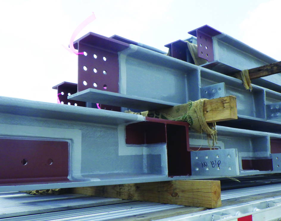
Hot-dip galvanising creates a metallurgical bond between zinc and steel. When executed correctly on a properly prepared surface, this bond is incredibly robust. However, several factors in the galvanising process can create a weak and unreliable substrate that may be unsuitable for supporting a safety-critical EPFP system. It is crucial to understand that these issues are not restricted to EPFP alone; they are a fundamental concern for all high-build coating systems that rely on a strong foundation to function. An example of galvanised steel section with EPFP applied is shown below in Photo 1.

This article will explore:

1. The inherent risks associated with galvanising including excessive thickness, metallurgical defects, and inadequate repair methods that can compromise the bond and ultimately could detract from the overall durability of the system.

2. This article will argue that the best practice is the direct application of EPFP paint systems to properly prepared steel substrates as a correctly installed EPFP system can give a comparable durability range. Therefore, galvanising should only be considered as a substrate for EPFP when there are no other design options available, and even then, only with additional (stringent) quality control measures that may go beyond typical industry/project expectations. This article will explore the inherent risks associated with galvanising including excessive thickness, metallurgical defects, and inadequate repair methods that can compromise the bond and ultimately could detract from the overall durability of the system.

2. The Challenge with Galvanising

The ability of a galvanised coating to support an EPFP system can be severely impaired by several influencing factors:

•Excessive galvanising thickness: The primary source of impairment.

•Metallurgical defects: Inclusions and weak layers that may form during the galvanising process.

•Poor bonding: Initial or Inadequate surface preparation leading to a weak bond.

•Surface passivation: Post-galvanising treatments that can impair adhesion.

The “Thicker is Better” Concept

Standard galvanising specifications like ISO 1461 and ASTM A123 are written with no consideration that EPFP system may also get specified and are typically for corrosion protection, they do not consider any additional thick film coating such a EPFP system.

They often imply that exceeding the minimum with no consideration to maximum thickness is not a cause for concern. However, for EPFP applications, this is a dangerous misleading understanding. Experience has shown that as a galvanised coating thickness increases, its cohesive strength may decrease. The primary drivers for this excessive growth are the chemical composition of the steel—typically its silicon (Si) and phosphorus (P) content—and the thermal mass of the steel section [2].

• High Silicon and Phosphorus Content: Steel with high levels of silicon (particularly in the range of 0.04% to 0.14%, known as the “Sandelin range”) and phosphorus accelerates the growth of the zinc-iron alloy layers (eta, zeta, and delta).

• Uncontrolled Growth: Rapid growth results in a thick, brittle, and often friable zeta layer. Instead of a dense, tightly bonded coating, there is an increasing likelihood that a coarse crystalline structure which is inherently weak may result.

Therefore, a galvanised coating that is too thick—for example, exceeding 250 µm (microns)—may not be robust when coated with thick EPFP coatings. It may have micro-cracks and a high degree of internal stress resulting in voids and weak layers. When the EPFP is applied over this type of surface, the galvanised layer itself can delaminate due to stress imparted by the EPFP.

3.Setting Strict Limits

Therefore, a robust, well-written project specification should consider the standard galvanising process and procedure but, in addition, set its own quality control and quality assurance requirements. The following limits should be considered important:

• Upper Galvanising Limit: The galvanising thickness must be strictly controlled. Any measurements exceeding 250 µm should trigger a formal integrity assessment. Sections with thicknesses greater than 250-400 µm should be quarantined until additional quality control testing can give assurance of acceptability. This includes but is not limited to. Adhesion testing using both internationally recognised standards and EPFP manufacturers’ recommended procedures.

• Mill Test Certificates: Engineers and specifiers should always review the steel’s Mill Test Certificate (MTC) at the design stage. An MTC (specifically a Type 3.1 certificate as per ISO 10474) provides a detailed chemical breakdown. If the silicon and phosphorus levels are high, excessive galvanising growth could be considered predictable, and the required additional inspection protocols can then be implemented by the engineer early at the galvaniser’s facility.

4.Defects Which Could Impair Performance

Defects within the galvanising layer that may create points of failure.

• Ash and Dross Inclusions: Ash (zinc oxide from the zinc bath surface) and dross (iron-zinc particles from the bath bottom) can become entrapped in the coating. These inclusions can be poorly bonded, creating an area of instant non-adhesion for the primer and EPFP [3].

5.Process Factors which Could Impair Performance

Properties at the surface of the galvanising layer that may create immediate points of failure.

• Passivation and Quenching: Post-treatment of galvanised surfaces with chromates or water quenching is common. Water quenching creates a thin, weak layer of zinc oxides and hydroxides on the surface. Chromate treatments are often used for aesthetics.This layer is completely unsuitable for coating adhesion and should be prohibited in the project specification. Any steel that has been water-quenched should be rejected before an EPFP application.

• Use of Cold Spray Repair Compounds: Where surface defects are observed by the galvaniser, cold spray repair compounds may be used to improve the aesthetic appearance of the galvanising.

Note. These repair compounds are not compatible with EPFP systems and may lead to coating system delamination. Any items where cold spray repair compounds have been used should be rejected prior to EPFP system application.

6.High Film Builds: A Closer Look at the Implications

When a thick-film material like EPFP is applied over a cohesively weak galvanised layer, several critical issues could materialise.

1. Adhesion Failure: The primer for the EPFP system cannot achieve a proper bond to a galvanised surface which is contaminated with weak oxide layers or has incompatible treatments applied. The failure point is within the incompatible treatment in the case of cold spray repair compounds or between the primer and the galvanised steel.

2. Internal Stress: The EPFP can induce stress during cure, and a brittle or weak, over-thick layer may crack or delaminate.

7. Remedial Actions: No Half Measures

When non-conformances are found, the remedial actions need to be appropriate to the EPFP system application. The goal is not to “repair” the galvanising in the traditional sense but to create a sound substrate for the EPFP.

1. Quarantined: For issues like water quenching or thickness exceeding 250 µm to 400 µm, the section should be quarantined. Until quality assurance can be demonstrated.

2. Thorough blasting with appropriate media: For sections with excessive thickness (250 µm – 400 µm) or surface defects like ash, the only acceptable method of repair is to aggressively abrasive blast. The goal of a “sweep blast” is not merely to create a profile; it is to remove the defective and friable outer layers of the galvanising until a sound adherent zinc layer is exposed. If this means blasting through to harder alloy layers in localised areas, then the justification can be presented: “Lifetime expectation is met by the application of the EPFP system.” However, this must be brought to the client’s attention as a technical or engineering query, as it fundamentally changes the specification requirement.

3. Stop Inadequate Repairs: Standard galvanising repair methods, such as cold spray repair compounds detailed in standards like ASTM A780, or the use of zinc-based solders (“zinc sticks”), should not be accepted for surfaces receiving EPFP. These repairs do not possess the cohesive strength or compatibility with the EPFP system and could create a point of failure.

All galvanised steel specified for EPFP application should always be sweep blasted to remove surface contaminants and any weak oxide layer, providing an angular profile of 50-75 µm for the EPFP system to anchor against. This should be stated clearly in the specification.

8. Conclusion: A Call for Best Practice

The industry must shift its mindset. Applying EPFP over hot-dip galvanising introduces significant, unnecessary risk to a facility’s most critical safety infrastructure. The default specification should always be EPFP applied directly to appropriately primed steel prepared to the EPFP manufacturer’s requirements.

When galvanising is unavoidable, it must not be treated as a finished product but as a substrate in need of quality control and further preparation for the EPFP system.

To achieve a safe and reliable outcome, the following actions should be considered essential.

• Early Intervention: Review mill test certificates at the project’s outset to identify reactive steels and plan for heightened inspection.

• Specify Correctly: Write a detailed coating specification that explicitly prohibits water quenching and surface treatments and defines strict lower and upper thickness limits for the galvanising coating.

• Mandatory Surface Preparation: Mandate that all galvanised surfaces receive an aggressive sweep blast to remove weak layers and create a suitable surface profile before priming.

• Consult the Experts: Engage the EPFP manufacturer at the design stage to assist with specifications and inspection test plans (ITPs).

By prioritising the integrity of the substrate, we can ensure that these vital safety systems perform as designed, protecting assets, the environment, and, most importantly, lives.

References

1. https://www.glorysteelwork.com/2024/05/07/causes-and-control-methods-of-hot-dip-galvanizing-surface defects/#:~:text=If%20there%20are%20more%20active,layer%20grow%20rapidly%20and%20push.

2. Kestler., C. E. (n.d.). The Galvalume Sheet Manufacturing Process. In C. E. Kestler., The Galvalume Sheet Manufacturing Process.

3. https://steelprogroup.com/galvanized-steel/finish/defects-and-treatment/#:~:text=Ash%20staining%20is%20caused%20by,dipping%2C%20leaving%20a%20grayish%20stain.

Meet The Authors

Christian Stone, M.S., M.Phys., is a corrosion scientist and technical expert at Concrete Preservation Technologies (CPT) who specialises in the development of next-generation corrosion management systems, supports the use of cathodic protection worldwide, and is a leading expert in corrosion in RAAC concrete. Christian sits on a number of professional organisations, is a member of the Loughborough University RAAC Research Team and is currently undertaking further research on RAAC with Loughborough University.

Gareth Glass is a Director at Concrete Preservation Technologies (CPT), a position he has held since the inception of the company in 2005.  He has extensive experience in materials technology, durability and rehabilitation of structures with over 100 publications to his name in the area of corrosion protection. He obtained his PhD from the Corrosion and Protection Centre, University of Manchester.

Introduction

The term ‘ageing factor’ (sometimes referred to as ‘ageing constant’) for galvanic Anodes, was first coined by Sergi et al in ‘Monitoring results of galvanic anodes in steel reinforced concrete over 20 years’ in Construction and Building Materials, 2020 [1]. The principle behind this idea is that discrete measurements of galvanic current data from precast anode systems, when plotted on a logarithmic graph, could be fitted with a straight line. Therefore, they claim that their anodes exhibit a ‘half-life’ model with the current trending to zero, halving over set time intervals, the ‘ageing factor’. They further claim that when the anodic current density falls below a threshold, the anodes no longer adequately protect the steel reinforcement.

Modelling – Apparent Discrepancies

The first site analysed by Sergi et al. was a bridge in Leicester; current was measured. approximately 26 times for 12 individual patch-anodes from a single patch over 20 years. The initial description of the anodic current describes three distinct stages of relatively stable current output, each below the prior level: 0-6 years, 7-14 years and 15-20 years. This was described, at least in part, due to a drop in pH of the pore solution of the electrolyte. A half-life ageing constant of approximately 7 years over which the current would half was then generated by the plotting of the current readings on a logarithmic scale and a straight line being fit to the data [1]. The reason for the choice of a logarithmic scale is not fully explained, with decreases in surface area and depletion of lithium hydroxide being cited.

This concept was furthered in the next year in the Journal of Building Engineering (June 2021) [3], at the Corrosion Conference (November 2021) [4], Structural Faults and Repair Conference (2022), an ICRI webinar, ’Design Considerations for Galvanic Anodes’ (December 2022) [5], in the book Life-Cycle of Structures and Infrastructure Systems [6], and 3rd Conference & Expo Genoa (2024) [7]. Throughout these publications, ‘ageing factors’ were published for approximately 12 elements using precast Vector Corrosion Technologies (VCT) anodes and their precast precursors, and included both site and laboratory data. Of particular note was the ICRI webinar and the AMPP Italy Corrosion Conference white paper, where the half-life style ‘ageing-factor’ hypothesis was applied to non-precast anodes manufactured by other companies, including Concrete Preservation Technologies (CPT) and an ‘ageing factor’ was published for CPT’s hybrid anode, one that is initially powered externally before being wired galvanically, the DuoGuard^TM anode system [5,7]. The predicted ‘ageing constant’ published for these anodes was 2.9 years, and was compared unfavourably to the 11 year ‘ageing factor’ for their own products.

There were however, some significant changes made to use of this empirical model. Rather than being a model for some precast patch anodes manufactured by a single company and their precursor anodes the hypothesis was now being applied to anode arrays cast with a different geometry, embedded in a different cementitious material, located in the host concrete rather than a patch, and very importantly not activated using the same chemistry that was cited as a major cause of the exponential decay in the original paper [1]. DuoGuard^TM is activated chemically in such a way that the activator is not depleted but recycled, continually drawn back to the anode. Therefore, the theoretical underpinnings cited by the authors do not appear to hold for these anodes. This has led to the need for a closer look at this model and whether it can tell us anything about the behaviour of these anode systems or whether the model can reliably predict the behaviour of CPT anodes.

In order to understand this model, it is important to first explore the stated and hidden axioms behind the hypothesis and how these lead Sergi, Whitmore and others to interpret their data in such a way. In this section, we will place to one side the fact that there is no stated theoretical underpinning to the choice of a logarithmic scale and allow for the strength of the predicted current data to judge
its veracity.

Half-Life Theory Axiom – There is A Set, Minimum Current Threshold For the Protection of Steel In Concrete

The corrosion risk of steel is due to its environment. This should be a relatively uncontroversial statement, as it is known that steel in fresh concrete is passive and requires no cathodic protection, and steel in carbonated concrete has a lower corrosion rate on average than steel in chloride-rich environments [8]. Furthermore, corrosion rates can vary due to the exposure to moisture, availability of oxygen and be changed by coatings applied to the steel. It is therefore reasonable to assume that the amount of protection steel in concrete requires for protection is a product of its environment.

Although the authors do acknowledge the importance of chloride in the amount of current needed to protect steel in concrete [7], they ignore many of the other factors. This inherent complexity is why it is often much easier to measure changes in the steel due to protection rather than purely the current output of the system. Such measurements are common with impressed current cathodic protection (ICCP) systems that use ISO 12696:2021 [9], which gives steel potentials in the immune region and polarisation held in the steel. originating from Mixed Potential Theory [10,11], as criteria for protection. Within galvanic cathodic protection (GCP), it is  common to track the depolarised steel potentials [12] to measure changes in corrosion risk, polarisation [13] and corrosion rates [14,15]. These measure the effect of the anodes on the steel rather than the output alone to determine the level of protection achieved.

Comparison of Anode Systems

This is further complicated by the fact that some anode systems are installed in different ways, leading to varied current spread. It matters very little how much current an anode produces if it is not reaching the at-risk steel it is installed to protect. To explain this concept more clearly, two anode systems for patch repair will be compared: a precast anode designed to be tied onto the reinforcement in a patch and a patch anode that is installed into a putty in the periphery of the patch, away from a single steel rebar. Below CPTs precast anode RebaGuard^TM and drilled anodes PatchGuard^TM can be seen. RebaGuard^TM is similar to the anodes installed in many of the author’s works.

The steel being protected by patch anodes is the steel outside of the patch, as the steel in the patch is in fresh, alkaline, contaminant-free concrete. The precast anodes are tied to the steel within the patch. It is not difficult to see that it is likely that a large portion of the current will take the easiest path between the zinc and the steel, to the reinforcement onto which it is tied. The current that does exit the patch must avoid taking the easiest path, passing through the interface between the patch and the host concrete, which will have a resistance and spread to the steel outside of the patch which is at some distance from the anodes. These anodes can and do work, but it is unlikely that all the current they produce is available to the steel they are protecting.

The PatchGuard^TM anode is installed into the periphery of the patch, in the host concrete into a conductive putty, much closer to the steel it is designed to protect. Unlike the precast anodes, it is not tied to a single reinforcement, and the current will therefore more easily spread to the at-risk reinforcement. Furthermore, due to the increased resistivity of most patch materials and the resistive interface of the patch making current flow into the patch more difficult, it will favour passing current to the steel outside the patch rather than within the patch. It is therefore logical to think that the current from this PatchGuard^TM anode will protect the rebar much more efficiently than the precast anode. Having the same current requirement for each of these anodes is illogical.

The validity of their threshold may be tested using the author’s data. The first work published in this series was the 20-year data from a ‘bridge in Leicester’ [1]. This site is a site which staff at CPT is quite familiar, and many senior members of staff were present at the installation of these anodes. Though the paper claims that after 20 years that the anodes are reaching the end of their life, with the current output dropping under their threshold for protection at approximately 14.5 years. In a statement to the Cathodic Protection Association (CPA) from March 2023 by CPT [16], it was shown that in 2015, ten years after the installation of the anodes, there was cracking in the element following the line of the reinforcement extending from the repairs. This is not a measure of success in a galvanic anode system and shows a flaw in their current threshold.

Potential Measurement Error – Taking Current Data From A Responsive System

One of the most important concepts with galvanic anodes is their responsive behaviour [17,18]. The driving voltage, as long as the anodes are activated, is due to the galvanic series and therefore can be approximated as constant; the current delivered to the steel is therefore largely dependent on the resistivity of the electrolyte in the circuit, the concrete. So, when the concrete is wet, full of ions, warm, etc, the circuit has a lower resistance and the cell between the zinc and the steel produces a higher current. This is a part of the draw of these anode systems as they give a level of protection which changes with the corrosion risk of the environment.

One of the issues that comes with this fluctuation in current is that when the anode currents are measured infrequently without other corresponding data, such as the weather. Steel polarisation or natural steel potentials – the data can be misleading. Currents taken on wet and warm days may be much larger than those taken on dry and cool days, which can make seeing trends in current output difficult, unless Adequate data is collected.

Furthermore, anodes installed into wet patches, or into slow-curing putties may have initial currents which are atypical due to the moisture surrounding the anode, decreasing the resistance between the zinc and the steel. In CPT’s anode systems, the putty may take many years to cure, a design feature to initially provide a larger current to aid in the passivation of the steel due to the reduction reactions at the steel surface producing hydroxide ions.

This ageing constant generated for CPT DuoGuard anodes was created from a few data points using anodic current data from
only the first nine years of the galvanic protection [7]. This was during the period when the putty was curing. This may have led
to some inaccuracies in predicting the long-term behaviour of these anodes.

Whiteadder Bridge – Duoguard Hybrid
Anode System CASE Study

The data used by Sergi et al to calculate the ageing factor for DuoGuard^TM anodes was taken from data published from Whiteadder Bridge in the UK [17].Here, two zones of anodes
were installed within a proprietary putty in regularly spaced,
drilled holes, and wired together to form arrays which protect the upper and lower portions of the structural element supporting the span of the bridge over a river. The anodes were installed to counteract the corrosion issues caused by de-icing salts and moisture ingress, including tidal flooding of the river.

The anodes were initially powered until at least 50kC of charge had been passed for every square meter of steel surface area to realkalise the steel environment, utilising the zinc’s ability to pass much higher currents than MMO titanium anodes when powered, and then connected directly to the steel via a junction box. Reference electrodes were installed in the zones, and the current output of the anodes alongside the reference potentials were measured by a data logger installed in an enclosure. This gives a constant stream of data, far in excess of those sites of similar ages used in the work by Sergi and Whitmore.

The element has been protected for 18.5 years now without the need for any maintenance beyond the replacement of SIM cards in the enclosure which transmit the data wirelessly to our office, and has been monitored with over 100,000 data points collected over the first 17.5 years of protection in each zone and over 1,000,000 data points collected in sum. The data used for the predicted 2.9-year ageing factor found in the AMPP Italy white paper [7] was taken from the first 9 years of data [17], which was not the most recent publicly available data set at the time [18] and appears to include only a small number of data points. It is unclear how these data points were selected. Due to the initial charging of the anodes, the authors claim that it would be expected that such anodes would likely have a decreased life due to having to pass a large amount of current early in their design life [7].

Although this model is now used in specifications and design documents worldwide, this will be the first predictive test of their empirical model and, importantly, a test of whether this model can be applied to anodes other than their own, for which they likely have a greater abundance of data. The aim of the following section is to analyse the predictive power of this model using data from the CPT site used in their analysis using the most recent data collected which presumably they had little access to.

Site Data – Responsive Behaviour

Below are the current and the polarised steel potentials for the lower zone of anodes installed on Whiteadder Bridge above, the same data used in the author’s work [7,17], but now with an additional 8 years of data. The red line is the galvanic current data showing the characteristic responsive behaviour with currents rising and falling in yearly cycles due to temperature changes and peaking during periods of increased moisture due to rainfall or flooding. This supports the theory that current is being driven in these anodes due to changes in resistance in the concrete electrolyte. The blue line is the polarised steel potential. When the current increases, we see a corresponding peak in the steel potential as the current generates a polarisation in the steel. Polarisation is a sign of steel passivity, with more passive steel polarising more easily than corroding steel. A green line has been added to show that over time the steel potentials are trending less negative, an indication of increased steel passivity.

The first few years of the data do show an increased current output from the anodes. As was previously stated, this is likely due to the putty into which the anodes were installed curing. After this period, the current appears to become more stable and respond to changes in resistivity from a relatively stable baseline. Taking a closer look at the data from around 9 years after installation, we can see the current from both zones increases due to fluctuations in temperature during the day as well as throughout the year. This response to corrosion risk with increased protection is one of the hallmarks of a naturally smart corrosion management system that is driven by electrochemistry.

After flooding and rainfall, we can see that not only does the current increase due to the moisture ingress, but it also falls slowly as the moisture evaporates, leading to increased protection during the entire period of increased risk. Furthermore, some of the peaks in current seen during periods of increased moisture are larger than

the initial anode current, indicating that the current output is not being primarily driven by a build up of corrosion products or a depletion in activator for these systems but a reaction to the environment and the corrosion risk.

Testing he Predictive Power of The Half-Life ‘Ageing Factor’

In order to test the predictive power of the model, we must choose a null hypothesis against which it will be compared. The simplest null hypothesis would be that the median current the system was producing between 8 and 9 years, the last year of the data set utilised by the authors, stays constant. This appears to be a fair null hypothesis to test their predicted values against, as one predicts a decrease and the other predicts no decrease in current.

The authors published a half-life ‘ageing factor’ of 2.9 years, where the current halves every 2.9 year period. Here we have plotted the predicted values for each hypothesis against the data collected from the site during the period from year 8 to year 17, approximately 3 ageing factors or an expectation that the current, if the model is correct, will fall by more than 87.5%. A log current graph was chosen to transcribe the half-life model data into a straight line in a similar fashion to that employed by Sergi in
his work.

As can clearly be seen, the values predicted by the ‘ageing factor’ model (red) diverge from those measured on site over time, whereas the constant current model fits the data much more closely. This becomes evident when the mean squared error (MSE) of each predicted data set is measured; with the half-life hypothesis having an MSE of 0.237 mA² and the MSE of a simple constant value
model being 0.0135 mA², an order of magnitude smaller.

The error is likely due to a misunderstanding of how these anodes will behave differently over time due to their activation chemistry and presuming that the same methodology should be employed without testing other hypotheses, leading to the authors choosing to fit the same exponential decay that fit their own data. A simple change in their methodology to presume an exponential decay overlaying a more stable pattern can lead to a much better fit in the data and a lower MSE over the previously available data.

Below is an empirical model presuming a decay plus a constant current calculated using the first 9 years of data only. It should be noted that this is not a lifetime predictive model for these anodes, which will depend on many factors, as the anodes will not continue protecting the steel indefinitely and it is expected that when the volume of the anodes reduces beyond a threshold the ratio of zinc to steel surface areas will be insufficient to pass the same current. This fact in included in the design calculations of these anode systems. This is also not an endorsement of current being used as a benchmark for anode performance. However, as around 7% of the anodes on this site have currently been consumed, in the lifetime provided for this system it is unlikely to reach this threshold and this basic model may suffice, depending on environmental conditions. Therefore, over this limited time period, a relatively stable current may be used as changes in surface areas are relatively slow due to the anode geometry chosen by CPT and the activator should continue to keep the zinc active. An initial period of higher current due to the resistivity drop from the curing of the putty is also included in this limited model.

We believe that much of the error in the predicted value of the ageing term is due to the presumption that the overall behaviour would be similar. However, the difference in the activators used to keep the anodes active may lead to differing behaviour giving precast anodes an exponential decay of current to zero. This depletion in their activator, may lead to the amount of protection being in a large part dependent not on the amount of zinc but rather on the amount of activator utilised. Activators such as lithium hydroxide are consumed, may be leached away from the anodes, and carbonate after manufacture. Anodes activated in similar ways to PatchGuardTM and DuoGuard^TM are likely to age very differently, as the availability of activator will not deplete in the same fashion and are therefore unlikely to show the same ageing characteristics. This can be seen clearly by calculating their hypothetical ageing constant using the data from years 8-17 using the same method as Sergi et al. Here we calculate the ageing constant over which the current is halved to be over 36,000 years. This is plainly absurd, as the zinc will be completely depleted after around 100-250 years. The underlying ageing of CPT anodes is therefore very unlikely to be exponential in nature.

Conclusions

It is clear from this data that the major factor driving the current output of CPT’s discrete anodes, is changes in the resistivity of the environment. After 17 years, the current was still responding strongly to changes in moisture, producing currents in excess of the median galvanic current from the first year of installation when moisture ingress reduces the resistivity of the environment. Precast anodes, such as the type used in the creation of the half-life model, may also be limited by a second factor, the depletion of their activator. This is concerning as these anode types are very popular worldwide and are often sold based on a mass of zinc, when, without sufficient activator, that mass of zinc will not be fully utilised. With lithium hydroxide as an activator, the mass of the activator would likely need to be much greater than the mass of zinc. It is likely, therefore, that only a portion of these anodes will be sufficiently activated before the current declines substantially.

Due to the depletion of activator, some form of ageing term may well apply to VCT style products as stated by their authors. However, due to this hypothesis failing to accurately predict the behaviour of other anode systems, it should be avoided in all specification documents as it may be unique to a certain set of products. It is important to ensure that clients are getting the same level of protection from anodes sold as equivalents in the market.

References

[1] G. Sergi, G. Seneviratne, D. Simpson, Monitoring results of galvanic anodes in steel reinforced concrete over 20 years, Construction and Building Materials, Volume 269, 2021, 121309, ISSN 0950- 618, https://doi.org/10.1016/j.conbuildmat.2020.121309.

[2] G. Sergi, Galvanic Corrosion Control of Reinforced Concrete: Lessons Learnt from 20 Years of Site Trials, ICorr presentation, Aberdeen, 30/03/2021, https://www.icorr.org/wp- content/uploads/2021/06/2021-03-30-ICorr-Aberdeen-Event-ICorr-Aberdeen-Presentation-30-03-21- Dr-George-Sergi-Vector-Corrosion.pdf 2021.

[3] G. Sergi, G. Seneviratne, D. Simpson, Monitoring results of galvanic anodes in steel reinforced concrete over 20 years, Construction & Building Materials, 269, 121309 2021.

[4] D. Whitmore, G. Sergi, Long-term monitoring provides data required to predict performance and perform intelligent design of galvanic corrosion control systems for reinforced concrete structures, Corrosion 2021, AMPP, Paper No. 16792, 2021.

[5] D. Whitmore, Design Considerations for Galvanic Anodes, ICRI webinar, December 2022.

6] G. Sergi, Life extension of existing steel reinforced structures by simple cathodic protection techniques for sustainable durability, Life-Cycle of Structures and Infrastructure Systems – Biondini & Frangopol (Eds), ISBN 978-1-003-32302-0 2023.

[7] G. Sergi, P. McCloskey, D. Simpson, Long-term performance of galvanic anodes for steel reinforced concrete, 3rd Conference & Expo Genoa 2024, AMPP Italy,https://www.vector- corrosion.com/assets/page_renderer/Sergi_George-Extended_Abstract.pdf, 2024.

[8] L. Bertolini, B. Elsener, P. Pedeferri, & R. Polder, Corrosion of Steel in Concrete: Prevention,Diagnosis, Repair. Corrosion of Steel in Concrete: Prevention, Diagnosis, Repair, 1–392. 2005 https://doi.org/10.1002/3527603379.

[9] ISO BS EN 12696:2022.

[10] G. K. Glass, A. M. Hassanein, N. R. Buenfeld, Monitoring the passivation of steel in concrete induced by cathodic protection, Corrosion Science, Vol. 39, No. 8, pp. 1451-1458, 1997.

[11] C. Stone, G. K. Glass, Assessment Criteria For The Electrochemical Protection Of Steel, Australasian Corrosion Association Conference, Cairns, November 2024.

[12] Standard Test Method for Corrosion Potentials of Uncoated Reinforcing Steel in Concrete, ASTM C876 22b, October 2022[11] National Highways 5700 Series.

[13] C. Christodoulou, C Goodier, S. A. Austin. Site performance of galvanic anodes in concrete repairs. Concrete Solutions-Proceedings of Concrete Solutions, 5th International Conference on Concrete Repair 2014 Aug 18 (pp. 167-172). 2014.

[14] Corrosion of steel in concrete: investigation and assessment, BRE Digest 444, 2000, ISBN 860813615.

[15] Electrochemical tests for reinforcement corrosion, Concrete Society Technical Report 60, 2024.

[16] G. K. Glass, Statement to the Cathodic Protection Association, SCA technical Meeting, March2023.

[17] D. Bewley, High-power, low-maintenance, hybrid corrosion protection, Bridge construction and repair, Concrete, Oct 2016, pp. 25-27 2016.

[18] D. Bewley, C. Stone, Long-term monitoring of innovative corrosion control system yields fascinating results, Concrete, Volume 57, Issue 5 June 2023.

Editor’s Note

This Journal provides a platform to all to present their investigations and research. It is not the intention to endorse particular products and readers must satisfy themselves in regard to their applicability and their particular needs.